
The stress-strain curve is the plot of stress (σ = F / S0) against strain (ε = ΔL / L0) measured in a tensile test. It gives you the modulus of elasticity, the yield strength, the ultimate tensile strength, the elongation and the toughness of the material. The same curve applies to a structural steel, an aluminum or a plastic. What changes is its shape, and that shape tells you how the material will behave in service.
30-second summary:
- Axes: stress σ = force ÷ original area, in MPa; strain ε = elongation ÷ original length, dimensionless or in %.
- Reading the curve: straight (elastic) portion, yielding, work hardening, maximum point, necking and fracture.
- Two curves: the engineering curve uses the original area and drops after the maximum point; the true curve uses the instantaneous area and keeps rising.
- In Brazil: CA-50 rebar is accepted on the basis of the test curve (ABNT NBR 7480:2024, the Brazilian standard for steel reinforcing bars), and structural design uses the idealized diagrams of ABNT NBR 6118:2023 (the Brazilian standard for the design of concrete structures).
What the stress-strain curve is and how it is obtained
The curve comes from the tensile test. A universal testing machine clamps the test specimen between two grips and pulls it at a controlled rate, usually until it fractures. During the test, the load cell measures the force F and the extensometer, attached to the specimen, measures the elongation ΔL over a marked length, the gauge length L0. The raw record is a force-elongation curve.
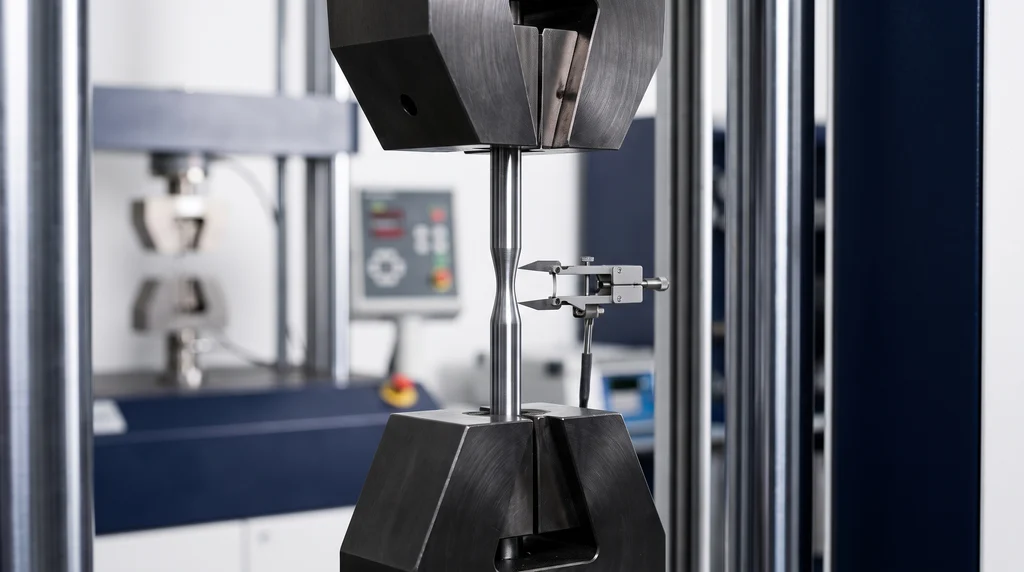
The photo shows a steel specimen held in the wedge grips of the universal testing machine, with the extensometer attached to the gauge section: this setup produces the force and elongation readings that make up the curve.
This raw curve is not yet a material property: a thicker specimen needs more force, and a longer one stretches more millimeters. To compare tests on specimens of different sizes, the software divides the force by the original cross-sectional area, S0, and the elongation by the original gauge length, L0:
- Engineering stress: σ = F / S0. With force in newtons and area in mm², the result is in N/mm², which is the same as MPa.
- Engineering strain: ε = ΔL / L0 = (L − L0) / L0. It is dimensionless (mm/mm); multiplied by 100, it is expressed in %.
These are the definitions given in ASTM E646 and used by ISO 6892-1 (ABNT NBR ISO 6892-1:2024 in Brazil), which specifies the tensile test method for metals at room temperature (10 °C to 35 °C). The plot of σ on the vertical axis against ε on the horizontal axis is the stress-strain curve. The term "engineering" means that S0 and L0 are held constant throughout the test, even after the actual cross section starts to shrink. This choice has consequences that show up later, in the comparison with the true curve.
The curve separates two kinds of deformation. Elastic deformation is reversible: it disappears when the load is removed. Plastic deformation is permanent. Depending on the type of loading, deformation can be tensile, compressive, shear or torsional; the curve in this article is the uniaxial tensile one, the most widely used to characterize materials.
How to read the stress-strain curve step by step
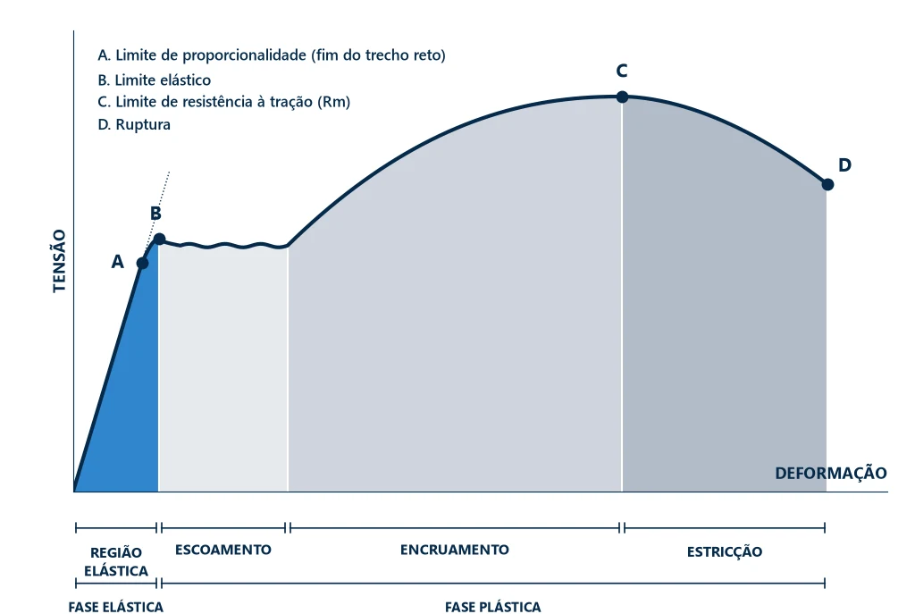
The curve of a ductile metal, such as a low-carbon steel, goes through four regions in sequence: elastic, yielding, work hardening and necking. The graph below shows these regions on a typical curve, with four marked points: A, the proportional limit, where the curve stops being straight; B, the elastic limit, just above it; C, the ultimate tensile strength; and D, fracture. The following items walk along the curve from left to right.
Elastic region and Hooke's law
At the start of the curve, stress and strain increase in the same proportion. This portion obeys Hooke's law, σ = E·ε, and the slope of the line is the modulus of elasticity (or Young's modulus), E = Δσ / Δε. The modulus measures stiffness: the higher it is, the less the material deforms under the same stress. In metals it depends on the strength of the bonds between atoms and hardly at all on the microstructure; that is why an annealed steel and a quenched steel have practically the same E, around 207 GPa. In steels, this portion ends at a strain on the order of 0.1% to 0.2%; on a curve that runs to 25%, it hugs the vertical axis, and to read E you need to zoom in on the beginning of the graph.
As the specimen stretches, it also gets thinner. The ratio of lateral strain to axial strain, taken as positive, is Poisson's ratio: ν = −εtransversal / εaxial. In metals it lies between 0.25 and 0.35, and the theoretical maximum for an isotropic material is 0.5. Measuring it requires an axial extensometer and a transverse one.
Proportional limit and elastic limit
These are two different points, and confusing them is one of the most common mistakes. The proportional limit is the end of the straight portion: the highest stress at which σ is still proportional to ε. The elastic limit is the highest stress the material can withstand without retaining permanent deformation after unloading. A material can remain elastic after it stops being linear: elastomers and concrete behave this way.
In metals, the two points nearly coincide and are hard to measure, because they depend on the sensitivity of the extensometer. In the figure above they appear almost on top of each other: A, where the curve departs from the dotted line, and B, just above it. Since the curve can stop being straight before any permanent deformation appears, the proportional limit is, strictly speaking, equal to or below the elastic limit. Because of this measurement difficulty, standards use the yield strength as the criterion, explained next.
Yielding: yield plateau or 0.2% offset
Yielding is the onset of plastic deformation, and the stress at which it occurs, the yield strength, is the basis of structural design: the part is sized to work below it. How it is measured depends on the material.
With a plateau. Low-carbon steels, such as hot-rolled or annealed 1020, show a plateau: the stress reaches a peak, the upper yield strength (ReH), drops slightly, and the specimen stretches without the stress rising, at the lower yield strength (ReL). In this stretch, bands of plastic deformation, the Lüders bands, travel along the gauge length.
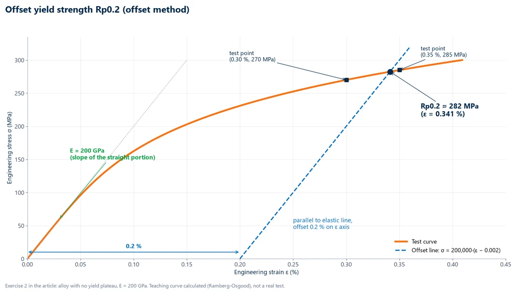
Without a plateau. In aluminum, copper, cold-worked steels and most alloys, the transition from elastic to plastic is gradual. In this case, the proof strength Rp0.2 is obtained by the offset method: a line parallel to the elastic portion is drawn starting from ε = 0.2% (0.002) on the horizontal axis, and the point where it intersects the curve is Rp0.2, the stress that leaves 0.2% permanent strain. The graph below shows the construction using the numbers from worked example 2, solved at the end of the article: E = 200 GPa and Rp0.2 of about 282 MPa.
Work hardening
After yielding, stress rises again with strain. This is work hardening (strain hardening): plastic deformation multiplies dislocations, the line defects whose motion produces deformation, and they begin to block one another, so more stress is needed to keep deforming. This is what raises the yield strength of a cold-drawn steel. Work hardening has a mathematical description, the Hollomon equation, presented in the section on the true curve.
Ultimate tensile strength (Rm)
The highest point of the engineering curve is the ultimate tensile strength, Rm = Fmax / S0, point C in the figure. Up to this point, deformation is distributed over the whole gauge length; the strain at this point is the uniform elongation, Ag. In the Brazilian rebar standard it appears with the symbol fst, and in older Portuguese-language texts as LR.
Rm is not the "fracture stress" of a ductile material: in such a material, fracture occurs later, at a lower engineering stress. Only in brittle materials do the two values coincide.
Necking
From Rm onward, deformation concentrates in one region of the specimen, which thins down to form a neck: this is necking. The area in this region starts to decrease faster than work hardening increases the strength, and the force needed to keep stretching drops. Since the engineering curve keeps dividing the force by S0, the calculated stress also drops, even though the material in the neck continues to harden.
Fracture, elongation and reduction of area
The last point of the curve, D in the figure, is fracture. After it, the two measures of ductility are taken. Elongation after fracture is A = (Lu − L0) / L0 × 100, with Lu measured by fitting the two broken halves together; since the elastic part recovers at fracture, A is plastic strain only. Reduction of area, the measured necking, is Z = (S0 − Su) / S0 × 100, with Su the smallest cross section at the neck.
Elongation depends on the gauge length: measured over 5 diameters, 10 diameters or 50 mm, the same material gives different numbers, because the neck weighs more in a short gauge length. Every value of A must be reported together with its L0.
Resilience and toughness: the areas under the curve
The area under the stress-strain curve is energy per unit volume (MPa multiplied by strain gives MJ/m³). The area under the elastic portion is resilience, the energy the material absorbs and returns when unloaded, measured by the modulus of resilience Ur = σe² / (2E). The area under the whole curve, up to fracture, is tensile toughness, UT = ∫σ dε: it combines strength and ductility, which is why a very strong but brittle material can have low toughness. Worked example 4 calculates both for 1020 steel.
Properties obtained from the curve
The table brings together what was covered in the previous items: each property, where on the curve it is read, the formula and the unit. It serves as a quick reference in the lab and when reading test certificates.
| Property | How it is read on the graph | Formula | Unit |
|---|---|---|---|
| Modulus of elasticity (E) | slope of the straight portion | Δσ / Δε | GPa |
| Proportional limit | end of the straight portion | direct reading | MPa |
| Elastic limit | highest σ without permanent deformation | test with unloading cycles | MPa |
| Yield strength (ReH, ReL, Rp0.2) | yield plateau or 0.2% offset | F / S0 | MPa |
| Ultimate tensile strength (Rm) | maximum point | Fmax / S0 | MPa |
| Uniform elongation (Ag) | strain at the maximum point | direct reading | % |
| Elongation after fracture (A) | final strain, without the elastic part | (Lu − L0) / L0 × 100 | % |
| Reduction of area (Z) | measured on the fractured specimen | (S0 − Su) / S0 × 100 | % |
| Resilience (Ur) | area under the elastic portion | σe² / (2E) | J/m³ |
| Toughness (UT) | area under the whole curve | ∫σ dε | J/m³ |
| Strain hardening exponent (n) | slope of log σv vs. log εv | σv = K·εvn | dimensionless |
Engineering vs. true stress-strain curve
The engineering curve uses the original cross-sectional area S0 and the original length L0 from start to finish. The true curve uses instantaneous values: true stress is σv = F / S, where S is the area at that instant, and true strain is εv = ln(L / L0), the sum of the small elongation increments, each divided by the length at that moment. The definitions are given in ASTM E646.
As long as deformation is uniform, one curve can be converted into the other without measuring the instantaneous area. Plastic deformation practically does not change the volume, so S·L = S0·L0, which gives:
- True stress: σv = σ·(1 + ε).
- True strain: εv = ln(1 + ε).
Both formulas are valid only up to Rm, the onset of necking. Beyond that point, deformation is no longer uniform, the neck cross-section is no longer given by S0·L0/L, and the conversion no longer makes sense. In the elastic region the two curves practically coincide, because the area barely changes; the difference grows with plastic deformation.
The numbers from exercise 3 show how large the difference is: a steel with Rm = 420 MPa and a uniform elongation of 20% is, at the same instant of the test, at σv = 420 × 1.20 = 504 MPa and εv = ln 1.20 = 0.182 on the true curve. The graph below compares the two curves for this steel: after Rm, the engineering curve drops until fracture, while the true curve keeps rising, drawn as a dashed line because it is only the trend.
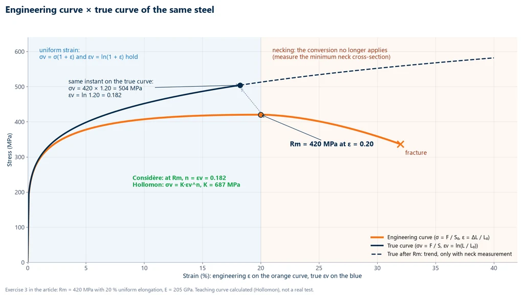
To obtain the true curve beyond Rm, you must measure the minimum neck diameter during the test, or correct the curve by simulation. The end point can be estimated from the reduction of area: εv,f = ln[1 / (1 − Z)]. In compression the opposite of tension happens: the cross-section increases, and the true stress is lower than the nominal stress.
Hollomon law and strain hardening exponent n
Between yielding and Rm, the true curve of many metals follows the Hollomon law well: σv = K·εvn. K is the strength coefficient, in MPa, and n is the strain hardening exponent, which measures how much the metal hardens as it deforms. In metals, n generally ranges from 0.1 to 0.5 (Dieter). It is determined according to ASTM E646-16(2024) or ISO 10275:2020, with a log-log fit: on a plot of log σv versus log εv, the law becomes a straight line with slope n. For low-carbon deep-drawing steel, the usual calculation range is 10% to 20% engineering strain. The article on work hardening covers the mechanism in detail.
Considère criterion
Necking begins when the strength gained through strain hardening no longer compensates for the loss of area: at the point of maximum force, the slope of the true curve equals the stress itself, dσv/dεv = σv. Applied to the Hollomon law, this criterion gives a simple result: at Rm, n = εv. A metal with a high n hardens more, delays necking and distributes deformation better, which explains why n is the number the sheet metal forming industry watches most closely in a sheet. From n and Rm you can also calculate K = Rm·(e/n)n, with e = 2.718, as in exercise 3.
Where each curve is used
The engineering curve is the one used in material certificates, product specifications and structural design, which works below the yield point; in that regime the difference between the two is negligible. The true curve comes into play when plastic deformation is large: in finite element simulation with nonlinear material models, in sheet metal forming and stamping, and in the study of work hardening. The table summarizes the comparison.
| Aspect | Engineering curve | True curve |
|---|---|---|
| Area used | original, S0 | instantaneous, S |
| Strain | ε = ΔL / L0 | εv = ln(L / L0) |
| After Rm | drops until fracture | keeps rising |
| Conversion | starting point | σ(1 + ε) and ln(1 + ε), only up to Rm |
| Typical use | certificate, specification, design | simulation, forming, work hardening |
Ductile and brittle materials
The shape of the curve separates materials into two groups. A ductile material, such as low-carbon steel, aluminum and copper, yields, work hardens, forms a neck and elongates considerably before fracture. Not every ductile material has a yield plateau: aluminum and copper move into the plastic regime gradually and are measured with the 0.2% offset method. The fracture of a ductile metal has a cup-and-cone appearance, with a high reduction of area, and the visible deformation gives warning before fracture.
A brittle material, such as gray cast iron, glass and ceramics, has an almost linear curve up to fracture: there is no yielding and no necking, and the ultimate tensile strength coincides with the fracture stress. The reason is that a crack propagates before dislocation motion can produce appreciable plastic deformation. The fracture is flat, perpendicular to the axis, and occurs without warning. The same material can change groups: body-centered cubic steels become brittle at low temperatures. Ductility and toughness are the properties that quantify this difference.
Stress-strain diagram of steel: 1020, CA-50 and NBR 6118
Steel appears in three versions of the diagram that should not be mixed up: the measured curve of a machinery steel such as 1020, the measured curve of a rebar for acceptance under the product standard, and the idealized diagram the designer uses in reinforced concrete calculations.
1020 steel
1020 steel is the classic example of a curve with a yield plateau. The values depend on the delivery condition, and the source must be cited along with them. For hot-rolled 1020 (round bar, 19 to 32 mm), the MatWeb data sheet gives a yield strength of 205 MPa, Rm of 380 MPa, elongation of 25% and reduction of area of 50%. For annealed 1020, Callister gives 180 MPa yield strength, 380 MPa tensile strength and 25% elongation.
Cold-drawn 1020 shows the effect of work hardening: the yield strength rises to about 350 MPa and the tensile strength to 420 MPa, but elongation drops to about 15% (typical values from the ASM table), and the yield plateau usually disappears. The modulus practically does not change with processing; see modulus of elasticity of steel.
CA-50 rebar (ABNT NBR 7480:2024)
CA-50 (a Brazilian reinforcing bar grade) is hot rolled and has a curve with a yield plateau and work hardening. ABNT NBR 7480:2024 (the Brazilian standard for steel bars for concrete reinforcement) requires three values from the tensile test:
- Characteristic yield strength: fyk ≥ 500 MPa, determined by the ISO 6892-1 test.
- Tensile-to-yield strength ratio: fst/fy minimum of 1.10 in the 2024 edition of ABNT NBR 7480 (it was 1.08 in the 2007 edition), according to the standard's table reproduced by the manufacturer in the CA-50 rebar data sheet.
- Elongation after fracture: A ≥ 8%, measured over 10 diameters.
The fst/fy ratio is a ductility requirement: it ensures that the bar, after yielding, still has a strength reserve before fracture. Exercise 5 shows the acceptance of a 12.5 mm bar using these three criteria. The bend test is a separate test.
Design diagram of steel (ABNT NBR 6118:2023)
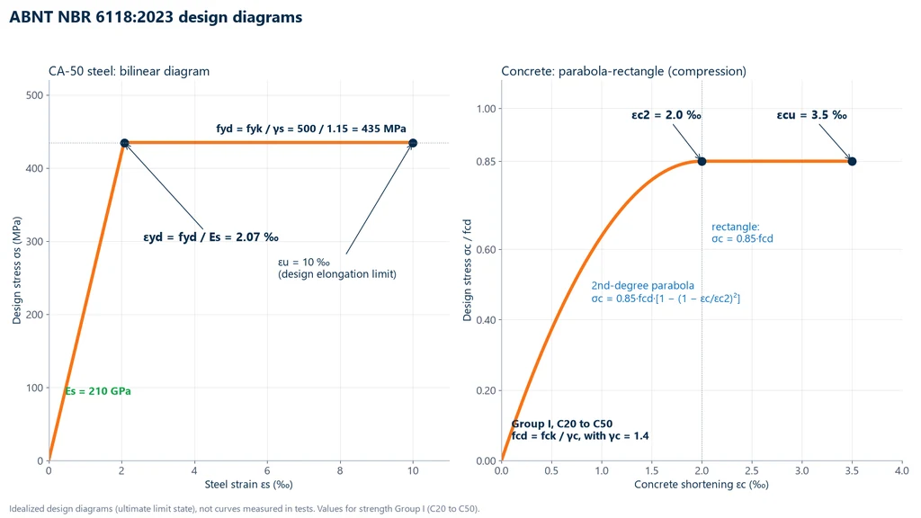
In reinforced concrete design, ABNT NBR 6118:2023 (the Brazilian standard for the design of concrete structures) does not use the measured rebar curve, but an idealized bilinear diagram: a straight line with modulus Es = 210 GPa (value assumed in the absence of testing) up to the design yield stress, followed by a horizontal plateau. The design stress is fyd = fyk / γs, with γs = 1.15; for CA-50, fyd = 500 / 1.15 = 435 MPa. The design yield onset strain is εyd = fyd / Es = 2.07 ‰, and the tensile elongation is limited to 10 ‰.
The same diagram applies to steels with or without a yield plateau, precisely because it is a design idealization, with a safety factor built in, and not a test curve. The actual work hardening of the rebar is left out of the calculation as a reserve. The graph of this diagram appears in the next section, alongside the concrete diagram.
Stress-strain diagram of concrete: parabola-rectangle
Concrete is tested and designed in compression. Its tensile strength is a small fraction of its compressive strength, and its behavior in tension is nearly brittle; in reinforced concrete, the concrete works in compression and the steel resists tension. The reference strength, fck, comes from the compression test of cylindrical specimens.
The concrete curve has no truly straight segment. For compressive stresses below 0.5·fc, ABNT NBR 6118:2023 allows a linear relationship with the secant modulus; the standard distinguishes the initial tangent modulus, Eci, from the secant modulus, Ecs (see modulus of elasticity of concrete). The assumed Poisson's ratio is 0.2.
At the ultimate limit state, the standard uses the parabola-rectangle diagram: a second-degree parabola up to strain εc2, followed by a horizontal segment up to the ultimate strain εcu, at an ordinate of 0.85·fcd. For Group I concretes (C20 to C50), the NBR 6118 values are εc2 = 2.0 ‰ and εcu = 3.5 ‰, and the parabola is σc = 0.85·fcd·[1 − (1 − εc/εc2)²]. The design strength is fcd = fck / γc, with γc = 1.4 under normal conditions. For Group II (C55 to C90), the parameters depend on fck.
The graphs below show the two design diagrams side by side: on the left, the bilinear CA-50 steel diagram, with fyd = 435 MPa, εyd = 2.07 ‰ and εu = 10 ‰; on the right, the Group I parabola-rectangle concrete diagram, with stress expressed as a fraction of fcd.
Polymers, ceramics and composites
Outside metals, the curve changes shape because the deformation mechanism is different. The main differences are summarized below, by material family.
Polymers
Polymers have a much lower modulus than metals: high-density polyethylene (HDPE) is around 1 GPa, compared with about 207 GPa for steel. There are three typical curve shapes:
- Semicrystalline thermoplastic (PE, PP, nylon): stress rises to a yield peak, drops, and a stable neck forms and propagates along the specimen as the chains align (cold drawing); at the end, stress rises again until fracture. Elongation reaches hundreds of percent.
- Brittle polymer (PMMA, polystyrene, Bakelite): an almost linear curve up to fracture, with an elongation of a few percent.
- Elastomer: an S-shaped curve, nonlinear from the start, with a low modulus and large recoverable elastic deformation.
Polymers are very sensitive to temperature and test speed. That is why ASTM D638-22 and ISO 527-1:2019 specify the speed, conditioning and specimen; two curves of the same plastic can only be compared under the same conditions.
Ceramics
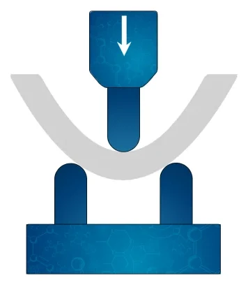
Alumina, silicon nitride and silicon carbide have a high modulus and a linear curve up to brittle fracture, without appreciable plastic deformation. Strength depends on the flaws introduced during manufacturing, which leads to large scatter between specimens. Because grips tend to break the part and any misalignment introduces bending, the strength of ceramics is rarely measured in tension: the 3-point or 4-point flexural test is used instead. Partially stabilized zirconia has a higher fracture toughness than the others, but it does not yield either.
Composites
Polymer matrix composites reinforced with carbon, glass or aramid fiber have, in the fiber direction, a practically linear curve up to fracture, with no yielding. The behavior is anisotropic: the curve measured at 90° to the fibers is different, dominated by the matrix. The fiber-matrix adhesion defines the failure mode, and the specimen follows dedicated standards, such as ASTM D3039.
Effect of temperature and strain rate
The same alloy gives different curves depending on the test temperature and speed. Higher temperature usually lowers the modulus, the yield strength and Rm, and increases ductility; lower temperature tends to do the opposite and, in body-centered cubic steels, to cause embrittlement. A higher speed raises the yield strength of many metals and, above all, of polymers. That is why ISO 6892-1 recommends method A, with strain rate control, which reduces the variation of rate-sensitive parameters, and the test report always states the condition used.
Typical material values
The values below serve as an order of magnitude to check whether a measured curve makes sense. To specify a material or accept a batch, the supplier's certificate or a test of the batch itself is what counts. The first table gives the modulus of elasticity at room temperature:
| Material | E (GPa) | Source |
|---|---|---|
| Steel (general) | 207 | Callister, Table 6.1 |
| Reinforcing steel, design value | 210 | ABNT NBR 6118:2023 |
| Aluminum | 69 | Callister, Table 6.1 |
| Copper | 110 | Callister, Table 6.1 |
| Titanium | 107 | Callister, Table 6.1 |
| HDPE | about 1.1 | Callister, Table 15.1 |
| Nylon 6,6 | 1.6 to 3.8 | Callister, Table 15.1 |
The second table gives the yield strength, tensile strength and elongation of metals, with the condition for each value. The Callister rows are for annealed material, and the source is given in parentheses:
| Material and condition | Yield strength (MPa) | Rm (MPa) | Elongation (%) |
|---|---|---|---|
| 1020 steel, hot rolled (MatWeb) | 205 | 380 | 25 |
| 1020 steel, annealed (Callister) | 180 | 380 | 25 |
| 1020 steel, cold drawn (typical, ASM) | 350 | 420 | 15 |
| Aluminum, annealed (Callister) | 35 | 90 | 40 |
| Copper, annealed (Callister) | 69 | 200 | 45 |
| Brass 70Cu-30Zn, annealed (Callister) | 75 | 300 | 68 |
| Titanium, annealed (Callister) | 450 | 520 | 25 |
| CA-50 rebar, minimums (ABNT NBR 7480:2024) | 500 | 1.10 × fy | 8 |
Solved exercises
The five exercises follow the curve in the same order as the article: elastic region, yielding, true curve, energy and acceptance of a real reinforcing bar.
Exercise 1: stress, strain and modulus of a steel
Cylindrical steel test specimen with d0 = 10.0 mm and an extensometer with L0 = 50 mm. At F = 15.7 kN, still in the linear region, the extensometer reads ΔL = 0.048 mm. Calculate σ, ε and E.
- Area: S0 = π × 10.0² / 4 = 78.54 mm².
- Stress: σ = 15,700 / 78.54 = 199.9 MPa, about 200 MPa.
- Strain: ε = 0.048 / 50 = 0.00096 (0.096%).
- Modulus: E = 199.9 / 0.00096 = 208,230 MPa, about 208 GPa, consistent with the 207 GPa given by Callister.
Exercise 2: Rp0.2 by the offset method
Alloy with no yield plateau, E = 200 GPa. Two points on the curve: (ε = 0.0030; σ = 270 MPa) and (ε = 0.0035; σ = 285 MPa). The offset line is σ = 200,000·(ε − 0.002).
- At ε = 0.0030, the line gives 200 MPa, below the curve; at 0.0035, it gives 300 MPa, above it. The intersection lies between the two points.
- Curve between the points, by linear interpolation: σ = 270 + 30,000·(ε − 0.003).
- Setting them equal: 270 + 30,000ε − 90 = 200,000ε − 400, so 580 = 170,000ε and ε = 0.003412.
- Rp0.2 = 200,000 × (0.003412 − 0.002) = 282 MPa. Check on the curve: 270 + 30,000 × 0.000412 = 282.4 MPa.
Exercise 3: from the engineering curve to the true curve, and Hollomon by Considère
Steel with Rm = 420 MPa and uniform elongation of 20% (ε = 0.20) at Rm.
- True stress at Rm: σv = 420 × (1 + 0.20) = 504 MPa.
- True strain: εv = ln 1.20 = 0.182.
- Considère: n = εv at Rm = 0.182.
- K = Rm·(e/n)n = 420 × (2.718 / 0.182)0.182 = 420 × 14.910.182 = 420 × 1.637 = 687 MPa.
- Check: K·εvn = 687 × 0.1820.182 = 687 × 0.733 = 504 MPa.
Beyond Rm these conversions no longer apply. The official n of a sheet is measured by a log-log fit, per ASTM E646 or ISO 10275; the Considère estimate is useful to check the order of magnitude.
Exercise 4: resilience and toughness of annealed 1020 steel
Data from Callister: σe = 180 MPa, Rm = 380 MPa, E = 207 GPa and elongation at fracture of 25%.
- Resilience: Ur = 180² / (2 × 207,000) = 32,400 / 414,000 = 0.078 MPa = 78 kJ/m³.
- Approximate toughness, from the area of a trapezoid: UT ≈ [(180 + 380) / 2] × 0.25 = 280 × 0.25 = 70 MJ/m³.
The elastic energy is almost a thousand times smaller than the total energy up to fracture: nearly all the toughness of a ductile metal comes from plastic deformation.
Exercise 5: acceptance of a CA-50 reinforcing bar
CA-50 bar (the Brazilian 500 MPa rebar grade) with φ = 12.5 mm and a nominal area of 122.7 mm². In the test: yield force of 66.3 kN, maximum force of 79.8 kN, gauge length 10φ = 125 mm and length after fracture of 143.8 mm.
- Yield: fy = 66,300 / 122.7 = 540 MPa, above 500 MPa.
- Strength: fst = 79,800 / 122.7 = 650 MPa; fst/fy = 650 / 540 = 1.20, above 1.10.
- Elongation: A = (143.8 − 125) / 125 × 100 = 15%, above 8%.
- For design: fyd = 500 / 1.15 = 434.8 MPa and εyd = 434.8 / 210,000 = 2.07 ‰.
The bar meets the three tensile requirements of ABNT NBR 7480:2024 (the Brazilian standard for steel reinforcing bars). With a maximum force of 79.8 kN, the test calls for a machine in the 100 to 200 kN range.
Common mistakes in reading and obtaining the curve
Besides the reading mistakes already pointed out throughout the article, four errors show up frequently in the lab and in test reports:
- Measuring strain from crosshead displacement. The crosshead adds grip slack and the deformation of the machine and load cell to the elongation of the specimen, and the modulus comes out far below the real value. For E and Rp0.2, use an extensometer; ASTM E646 requires class C or better per ASTM E83.
- Comparing curves obtained at different speeds or temperatures. In polymers, the difference can be larger than the difference between materials.
- Mixing units on the strain axis. Published curves give ε sometimes in %, sometimes in mm/mm; a factor-of-100 error in the modulus almost always comes from this.
- Taking the "allowable stress" from the curve. It is not a material property: it comes from the design code, based on the yield strength and a safety factor, such as fyd = fyk / 1.15 in NBR 6118 (the Brazilian standard for design of concrete structures).
Stress-strain curve standards
The curve is the same, but the method for obtaining it and the required values come from different standards depending on the material and the application. The table lists those cited in this article, with the current edition:
| Standard | Scope | Edition |
|---|---|---|
| ABNT NBR ISO 6892-1 | tensile testing of metals at room temperature (Brazilian adoption of ISO 6892-1) | 2024 |
| ISO 6892-1 | tensile testing of metals at room temperature | 2019 |
| ASTM E8/E8M | tensile testing of metals | E8/E8M-25 |
| ASTM E111 | Young's modulus, tangent modulus and chord modulus | E111-17(2025)e1 |
| ASTM E646 | strain hardening exponent n of metallic sheet | E646-16(2024) |
| ISO 10275 | strain hardening exponent n of sheet and strip | 2020 |
| ASTM D638 | tensile testing of plastics | D638-22 |
| ISO 527-1 | tensile testing of plastics, general principles | 2019 |
| ABNT NBR 7480 | steel for reinforced concrete (CA-25, CA-50, CA-60), Brazil | 2024 |
| ABNT NBR 6118 | design of concrete structures (design diagrams), Brazil | 2023 |
Machine for obtaining the stress-strain curve
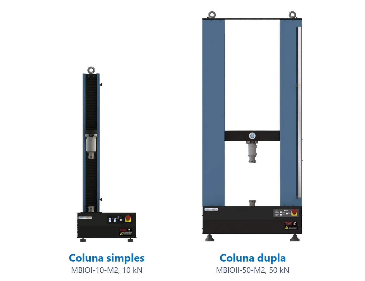
To obtain the curve, you need to apply force at a controlled rate, measure the force with a load cell sized for the test and measure elongation with an extensometer on the specimen itself, which is what gives a reliable modulus and Rp0.2. The Biopdi M2 universal testing machine is electromechanical and does all three: it comes in single-column models, from 200 N to 10 kN, and dual-column models, from 5 kN to 1,000 kN, with extensometers and the BioLab software, which plots the stress-strain curve and calculates modulus, yield strength, tensile strength and elongation. The panel below shows the machine, the role of each part in obtaining the curve and the grips used.
The universal testing machine in the tensile test
The M2 line has single-column models, from 200 N to 10 kN, and dual-column models, from 5 kN to 1,000 kN. Each part of the machine has a role in obtaining the curve:
- Moving crosshead pulls the specimen at the speed set by the standard
- Load cell measures the force F, class 1
- Grips: wedge, pneumatic, for threaded specimens or wires
- Extensometer measures ΔL over L0, for E and Rp0.2
- BioLab software divides by S0 and L0, plots the curve and calculates E, yield strength, Rm and A
- Control panel and emergency stop position and stop the test
Fixtures for the tensile test
The fixtures below are mounted on the same machine, depending on the specimen and the standard:
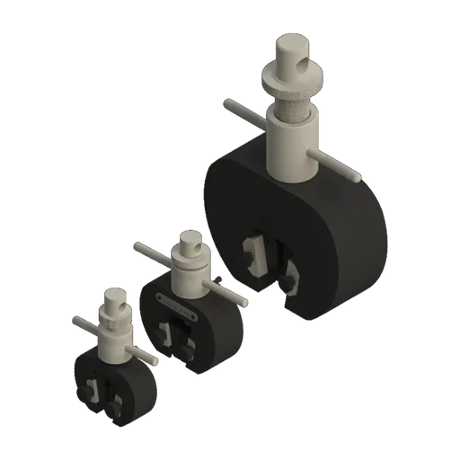 Wedge grip5, 20 and 200 kN
 Pneumatic wedge grip50 and 200 kN
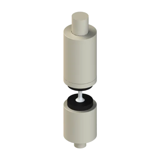 Grip for threaded specimensbolts and threaded test specimens
For reinforcing bars like the one in exercise 5, the recommended model is the 100 to 200 kN universal testing machine (MBIOII-200-M2). In the BioLab software, custom calculation formulas let you create your own quantities from force, position and extensometer, such as true stress and true strain up to Rm. The other capacities are on the universal testing machine page.
Other tests and technical references
Tests performed on the Biopdi universal testing machine







Related technical references
NBR 7480: requirements for CA-25, CA-50, CA-60 and CA-70 rebar steel, table and tests
ABNT NBR 7480:2024 (the Brazilian standard for steel bars and wires for reinforced concrete) sets the requirements for rebar: categories CA-25, CA-50, CA-60 and CA-70, minimum yield strength, fst/fy ratio, elongation, bend test, linear mass and sampling. The test methods come from ISO 6892-1 (ABNT NBR ISO 6892-1 in Brazil) for the tensile test and from ABNT NBR 17005 for the bend test.
Flexural test: 3-point and 4-point bending, how to calculate flexural strength, and standards
In a flexural test, a bar supported at two points is loaded until it fails. Learn 3- and 4-point setups, flexural strength and modulus formulas, NBR 12142 and ASTM D790.
NBR 5739 concrete compression test: fc calculation and the NBR 7222, NBR 12142 and NBR 6136-2 standards
ABNT NBR 5739:2018 (the Brazilian standard for concrete compression testing), reaffirmed in 2023, covers compression testing of cylindrical concrete specimens: continuous loading at 0.45 ± 0.15 MPa/s until failure and fc = 4F/(πD²), in MPa, to three significant figures. See what it requires of the machine and the specimen, the h/d correction, failure types A to G and the related standards: NBR 7222 (splitting tensile test), NBR 12142 (flexural tensile strength) and NBR 12118, withdrawn in February 2026 and replaced by NBR 6136-2:2026.
Frequently asked questions
What is the stress-strain curve?
It is the plot of stress (σ = F/S0) against strain (ε = ΔL/L0) measured in the tensile test. It gives the modulus of elasticity, yield strength, ultimate tensile strength, elongation and toughness of the material.
What is the formula for stress and strain?
Stress σ = F/S0, the force divided by the original area, in MPa; strain ε = ΔL/L0, the elongation divided by the original length, dimensionless. In the elastic region they are related by Hooke's law, σ = E·ε.
What is the formula for true strain?
εv = ln(L/L0) = ln(1 + ε), where ε is the engineering strain. True stress is σv = σ(1 + ε). Both conversions are valid up to the onset of necking, at the ultimate tensile strength (ASTM E646-16(2024)).
What are the types of deformation?
Elastic, which disappears when the load is removed, and plastic, which is permanent. By type of loading, there is tensile, compressive, shear and torsional deformation.
What is the difference between the engineering curve and the true curve?
The engineering curve divides the force by the original area and the elongation by the original length. The true curve uses the instantaneous area and length. After the ultimate tensile strength the engineering curve drops, because of necking, while the true curve keeps rising until fracture.
Why does the engineering curve drop after the ultimate tensile strength?
Because the cross-section of the specimen narrows into a neck and the required force decreases, while the calculation keeps dividing by S0. The material in the neck is actually still work hardening.
Are the proportional limit and the elastic limit the same thing?
No. The proportional limit is the end of the linear region; the elastic limit is the highest stress without permanent deformation. In metals they nearly coincide and are hard to measure, which is why standards use the yield strength, such as Rp0.2.
How do you find the yield strength when there is no yield plateau?
Draw a line parallel to the elastic region starting at 0.2% strain. The point where it intersects the curve is the offset yield strength Rp0.2.
What is the breaking stress of steel?
It depends on the steel. Hot-rolled 1020 has an ultimate tensile strength of about 380 MPa (MatWeb). Brazilian CA-50 rebar must have fyk of at least 500 MPa and an fst/fy ratio of at least 1.10 (ABNT NBR 7480:2024, the Brazilian standard for steel reinforcing bars). In ductile steel, fracture occurs after the ultimate tensile strength, at a lower engineering stress.
What does the stress-strain curve of concrete look like?
For design, ABNT NBR 6118:2023 (the Brazilian standard for design of concrete structures) uses the parabola-rectangle diagram: a parabola up to 2 ‰ and a plateau at 0.85·fcd up to 3.5 ‰, for Group I concretes (C20 to C50). The reference test for concrete is the compression test.
What is the difference between the curve of a ductile material and that of a brittle one?
A ductile material shows yielding, work hardening, necking and large elongation. A brittle one, such as gray cast iron, glass and ceramics, is almost linear until it breaks, and its ultimate tensile strength coincides with fracture.
What is the strain hardening exponent n?
It is the exponent in Hollomon's law, σv = K·εv^n, and measures how much the metal hardens as it deforms. In metals it typically lies between 0.1 and 0.5 and is measured per ASTM E646 or ISO 10275.