Hooke's law: formula, graph and solved problems

Hooke's law states that, within the elastic range, the deformation of a body is proportional to the force that causes it. For a spring, it is written F = k·x: the elastic force F (in newtons) equals the spring constant k (in N/m) times the deformation x (in meters). For materials, the same proportionality appears as σ = E·ε: stress equals the modulus of elasticity times strain.

In one sentence: Hooke's law states that, in the linear elastic range, force is proportional to deformation (F = k·x) and stress is proportional to strain (σ = E·ε), and it holds only up to the material's proportional limit, which is measured in the tensile test.

This guide covers both forms of the law. First come the spring, the graph, the spring constant and the experiment. Then come the form used in strength of materials, the generalized form for stresses in three directions, the limits of validity of the law, how the modulus of elasticity is measured on a universal testing machine, and seven solved exercises.

The photo shows a steel test specimen held in the grips of a universal testing machine, with the extensometer attached to the gauge length. This is the instrument that measures the very small deformations in the range where Hooke's law holds.

The table summarizes the two forms of the law, the relationship that links them, k = E·A/L, explained in the section on the spring constant, and the generalized form for parts under stress in more than one direction.

Form	Formula	Constant	Where it is used
Spring	F = −k·x	k, spring constant (N/m)	Springs, spring scales, high school physics
Materials	σ = E·ε	E, modulus of elasticity (GPa)	Tensile test, strength of materials, structural design
Bridge between the two	k = E·A/L	depends on the material (E) and the shape of the part (A and L)	Bars, cables and parts under axial load
Generalized Hooke's law (3D)	εx = [σx − ν(σy + σz)]/E	E and ν (and G = E/[2(1 + ν)])	Parts under stress in more than one direction, strain gauges, finite elements

What is Hooke's law

Hooke's law is the linear relationship between force and deformation in an elastic body. If a force of 10 N stretches a spring by 2 cm, a force of 20 N stretches the same spring by 4 cm. When the force is removed, the spring returns to its original length. This complete return is what defines elastic behavior.

This proportionality underlies many engineering calculations. It is what allows a spring to be used as a measuring instrument, in force gauges and spring scales, and what is used to size vehicle suspension springs and springs in mechanisms such as watches. A suspension spring with k = 15,000 N/m, compressed 10 cm by the weight of the car, exerts 15,000 × 0.10 = 1,500 N. In structures, the same law, written in terms of stress and strain, is used to calculate how much beams, columns and cables of bridges and buildings deform under service load, as long as they work in the elastic range.

The law is named after the Englishman Robert Hooke (1635-1703), a member of the Royal Society. In 1676, he published the discovery as an anagram, "ceiiinosssttuv", at the end of the book A Description of Helioscopes, and Some Other Instruments. It was a way of securing priority without revealing the idea. In 1678 came the solution, in the book Lectures de Potentia Restitutiva, or of Spring: "ut tensio, sic vis", meaning "as the extension, so the force". In the same text, Hooke writes that the force of any spring is in the same proportion as its extension.

The form used in engineering today came later. In 1807, Thomas Young described the constant that relates the stress and strain of a material, now called the modulus of elasticity or Young's modulus. The idea had already appeared in works by Euler (1727) and Giordano Riccati (1782). That is why the same law has two faces: the spring version, learned in physics, and the material version, measured in the laboratory.

Hooke's law formula

The Hooke's law formula for a spring is:

F = −k · x

The deformation x is the difference between the length of the deformed spring, L, and its free length, L₀: positive when the spring is stretched, negative when it is compressed. The table lists the symbols and their SI units:

Symbol	Quantity	SI unit
F	Elastic force, exerted by the spring	newton (N)
k	Spring constant	newton per meter (N/m)
x	Deformation, or extension: x = L − L0	meter (m)

Why the negative sign? It indicates that the elastic force acts in the direction opposite to the deformation. If the spring is stretched downward, the elastic force acts upward; if it is compressed, it acts to extend it back. That is why the elastic force is called a restoring force. The sign does not mean that k is negative. In most exercises only the magnitude matters, and the formula is used as F = k·x.

What does k mean? The spring constant is the force needed to deform the spring by 1 meter. A spring with k = 200 N/m needs 200 N to stretch 1 m, or 10 N to stretch 5 cm. The higher the k, the stiffer the spring.

Watch the units. The most common mistake in exercises is using the deformation in centimeters with k in N/m. Always convert: 5 cm = 0.05 m.

A stretched spring stores elastic potential energy, given by E_p = ½·k·x². This is the same energy the material returns when unloaded, the basis of the concept of resilience of materials.

Hooke's law graph

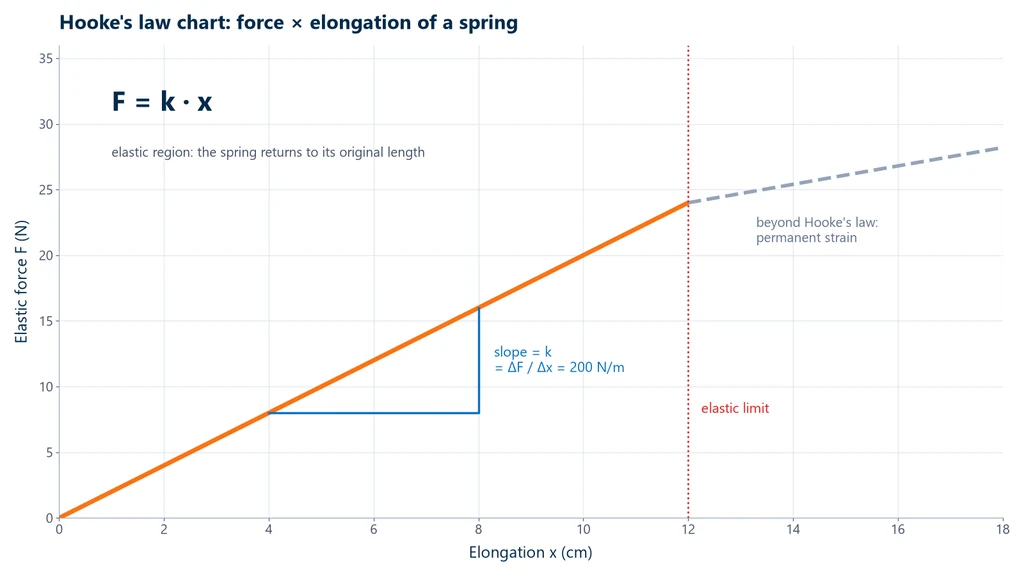
The Hooke's law graph is a straight line through the origin. The horizontal axis shows the deformation x; the vertical axis, the force F. Three readings come straight from the graph:

• The slope of the line is the spring constant: k = ΔF / Δx. Steeper line, stiffer spring.
• The area under the line is the elastic energy stored, ½·k·x² (the area of a triangle).
• The end of the line is the limit of the law, the proportional limit, detailed further on. Beyond it, the same force produces more deformation, and past the elastic limit the spring no longer returns to its original length.

The graph below shows these readings for a 200 N/m spring, which follows the straight line up to 12 cm of extension. Up to that point, doubling the force doubles the extension. After that, the curve flattens: the spring yields more than F = k·x predicts and is left with permanent deformation.

In the simulation below you can hang masses on a spring and watch this happen, and also apply stress to a test specimen of steel, aluminum, copper or polypropylene.

Spring constant: what makes a spring stiffer

The spring constant is not a property of the material. It is the stiffness of the part, and it depends on the material and the geometry. Two bars of the same steel, with the same cross section and lengths of 1 m and 2 m, have the same modulus of elasticity, but the 2 m bar has half the spring constant. For a bar under tension or compression:

k = E · A / L

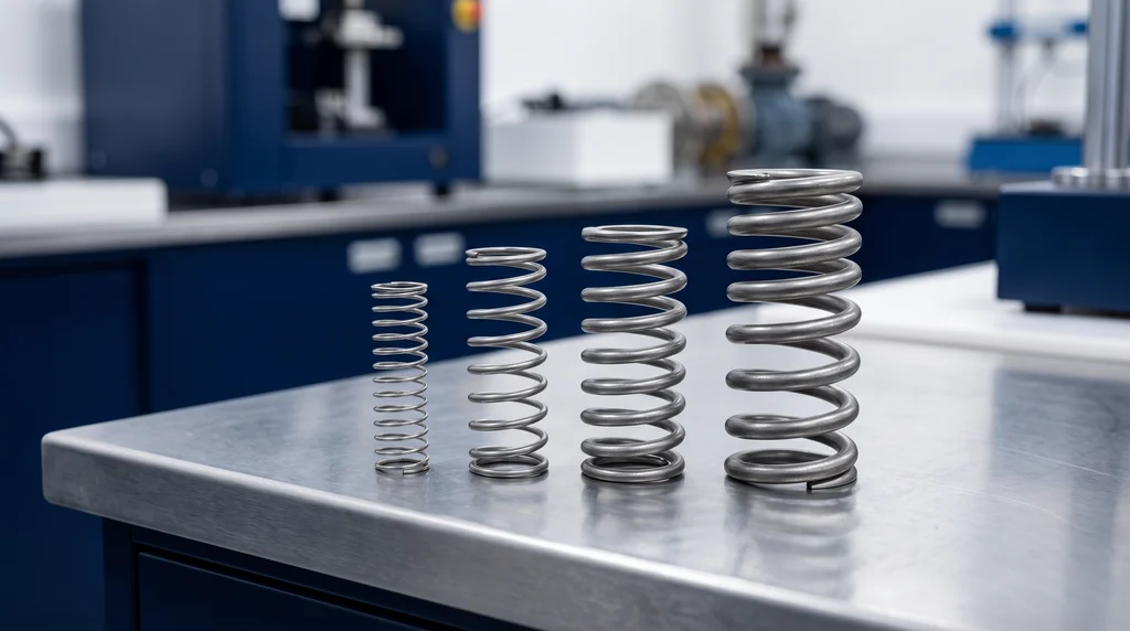
where E is the modulus of elasticity of the material (the stiffness of the material itself, covered in the section on σ = E·ε), A is the cross-sectional area and L is the length. In a helical spring, the wire works in torsion, and the constant depends on the shear modulus G, the torsional equivalent of E: k = G·d⁴ / (8·D³·n), with d the wire diameter, D the mean coil diameter and n the number of active coils. A thicker wire makes the spring much stiffer (the fourth power of d); a wider coil and more coils make the spring softer.

The photo below shows this effect in four steel helical springs: made of the same material, they range from the most flexible to the stiffest as the wire gets thicker.

Springs in combination. When two springs work together, the equivalent constant depends on how they are connected. In series, one after the other, both carry the same force and the deformations add up, so the assembly yields more than each spring alone. In parallel, side by side, both undergo the same deformation and the forces add up, so the assembly is stiffer. The table summarizes the formulas:

Combination	Equivalent constant	Effect
In series (one after the other)	1/keq = 1/k1 + 1/k2	Assembly softer than the softest spring
In parallel (side by side)	keq = k1 + k2	Stiffer assembly: the constants add up

Hooke's law experiment step by step

The classic experiment measures the spring constant of a spring with simple laboratory equipment:

1. Attach the spring to a vertical stand, with a scale next to it, and record the initial length L₀.
2. Hang a known mass, wait for the spring to stop moving and record the new length L. The deformation is x = L − L₀.
3. Repeat with larger masses (for example 50, 100, 150 and 200 g).
4. Calculate the force at each point, which is the weight: F = m·g, with g = 9.8 m/s² and the mass in kilograms.
5. Plot the F × x graph. If the points line up on a straight line through the origin, the spring obeys Hooke's law.
6. The slope of the line is k. With real data, which have scatter, calculate the slope by linear regression instead of using a single point.

The photo shows this setup: the spring attached to the stand, the calibrated masses hanging from its end and the scale next to it to read the length.

The main sources of error are reading the scale while the spring is still oscillating, parallax in the reading and using masses that are too heavy, which take the spring beyond its elastic limit. When removing the masses, check whether the spring returned to L₀: if it did not, the last points were already outside the law. The same reasoning, with far more precise instruments, applies to the tensile test on a universal testing machine.

Hooke's law in strength of materials: σ = E·ε

In engineering, comparing forces and extensions is not enough, because they depend on the size of the part. That is why Hooke's law is written in quantities that are independent of geometry:

• Stress: σ = F / A₀, the force divided by the initial cross-sectional area, in pascals (usually MPa).
• Strain: ε = ΔL / L₀, the extension divided by the initial length, dimensionless (or in %).
• Modulus of elasticity: E, the constant of proportionality, in pascals (usually GPa).

σ = E · ε

On the stress-strain curve, the modulus of elasticity is the slope of the initial straight portion. Unlike the constant k, it is a property of the material: it practically does not change with the shape of the part. Substituting these two definitions into σ = E·ε gives the elongation of a bar under axial load, δ = F·L / (E·A). This is the same relationship k = E·A/L seen in the spring constant section, written for elongation, and it is the most widely used equation in design within the elastic range.

Hooke's law also applies to shear, in the form τ = G·γ, with G the shear modulus. In isotropic materials, G, E and Poisson's ratio ν are related by G = E / [2(1 + ν)].

The table lists the three parameters for common metals. It shows, for example, that steel is about three times stiffer than aluminum: under the same stress, an aluminum bar deforms three times as much.

Metal	Modulus of elasticity E (GPa)	Shear modulus G (GPa)	Poisson's ratio ν
Steel	207	83	0.30
Nickel	207	76	0.31
Copper	110	46	0.34
Titanium	107	45	0.34
Brass	97	37	0.34
Aluminum	69	25	0.33
Magnesium	45	17	0.29
Tungsten	407	160	0.28

Room temperature values, from Callister and Rethwisch, Materials Science and Engineering (Table 6.1). The modulus of elasticity of steel is close to 200 GPa and varies little with carbon content and heat treatment. In polymers the value is much lower and varies with processing: polypropylene is around 1.1 to 2 GPa, polycarbonate around 2.4 GPa and low-density polyethylene between 0.1 and 0.5 GPa. For concrete, ABNT NBR 6118 (the Brazilian standard for the design of concrete structures) estimates the initial modulus from the characteristic compressive strength, E_ci = α_E·5600·√f_ck (in MPa), as explained in the article on the modulus of elasticity of concrete.

Generalized Hooke's law: stresses in three directions

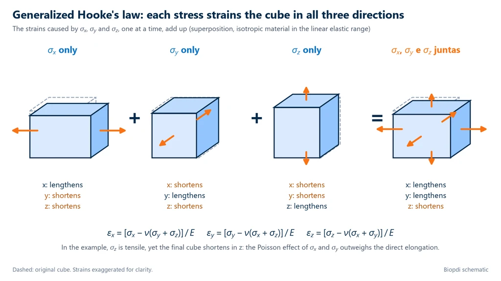
The generalized Hooke's law extends Hooke's law to the triaxial state of stress. In a linear elastic, homogeneous and isotropic material under small strains, each normal strain depends on all three normal stresses: each stress elongates the material in its own direction and, through the Poisson effect, shortens it in the other two.

The previous section dealt with one stress at a time: σ = E·ε in the load direction and τ = G·γ in shear. In a real part, a point is usually stressed in more than one direction, as in the wall of a pressure vessel, at the surface of a shaft or in a block compressed inside a die. The generalized law handles this case by superposition. It calculates the strain caused by σ_x alone, then the strain caused by σ_y and by σ_z, and adds them up. The constants are the same ones obtained in the tensile test: the modulus of elasticity E and Poisson's ratio ν. The consequence shows up in the tensile test itself, and the Strength of Materials slides from UFJF (Federal University of Juiz de Fora, Brazil) sum it up this way: "a uniaxial state of stress produces a triaxial state of strain".

The diagram below shows the superposition on an elementary cube. In the first three cubes, a single tensile stress acts alone: the cube elongates in its direction and shortens in the other two. In the fourth cube, all three act together, and each final dimension is the sum of the three effects. With the stresses in the example, the z dimension shortens even under tension in z, because the Poisson contraction caused by σ_x and σ_y outweighs the direct elongation.

The six equations for an isotropic material

Adding the three effects in each direction gives the three equations for the normal strains. The three shear equations are independent of them: each shear stress produces only the shear strain of its own plane.

• ε_x = [σ_x − ν(σ_y + σ_z)]/E
• ε_y = [σ_y − ν(σ_x + σ_z)]/E
• ε_z = [σ_z − ν(σ_x + σ_y)]/E
• γ_xy = τ_xy/G, γ_yz = τ_yz/G and γ_zx = τ_zx/G, with G = E/[2(1 + ν)]

The relationship between G, E and ν is derived step by step in the article on the shear modulus. The equations above, found in the Strength of Materials course notes from UFJF and UFF (Fluminense Federal University, Brazil), hold under these assumptions:

• Linear elastic behavior: all stresses below the proportional limit, covered in the next section.
• Small strains: this is what allows the effects to be added without one changing the geometry on which the other acts.
• Homogeneous and isotropic material: the same properties at every point and in every direction. Polycrystalline metals meet this in practice, because the grains are randomly oriented; wood and composites do not.
• Uncoupled effects: in an isotropic material, shear stress does not change the normal strains, and normal stress does not cause shear strain.

The most common mistake is to apply σ = E·ε direction by direction in a biaxial state. In the steel block of Exercise 6, with σ_x = 120 MPa and σ_y = −60 MPa, the uniaxial calculation gives ε_x 13% below the correct value, because it ignores that the compression in y elongates the block in x.

Matrix form: compliance and stiffness

The same equations fit into a matrix, which is the form used by finite element programs and calculation spreadsheets. In the compliance form, the strains are obtained from the stresses: {ε} = [S]{σ}. The table shows the normal stress block: each row is a strain, and each column is the contribution of one stress. It is the superposition of the diagram above, written term by term.

Strain	σx term	σy term	σz term
εx	1/E	−ν/E	−ν/E
εy	−ν/E	1/E	−ν/E
εz	−ν/E	−ν/E	1/E

The full matrix is 6 × 6, with the six stresses (σ_x, σ_y, σ_z, τ_yz, τ_zx, τ_xy) and the six strains. The shear block is diagonal: each shear strain depends only on its own stress, and the diagonal term is 1/G = 2(1 + ν)/E. The terms that would couple normal stress to shear strain, and shear to normal strain, are zero in an isotropic material.

Inverting the matrix gives the stresses from the strains: {σ} = [C]{ε}, the stiffness form. All the terms of the normal block carry the factor E/[(1 + ν)(1 − 2ν)], and the table shows what multiplies this factor at each position:

Stress	εx term	εy term	εz term
σx	1 − ν	ν	ν
σy	ν	1 − ν	ν
σz	ν	ν	1 − ν

In the shear block of the stiffness matrix, the diagonal term is the same factor times (1 − 2ν)/2, which equals G: we are back to τ = G·γ. For steel, with E = 200 GPa and ν = 0.3, the factor is 200/(1.3 × 0.4) = 384.6 GPa, and the normal block has 269.2 GPa on the diagonal and 115.4 GPa off the diagonal. Both matrices are on slides 11 and 12 from UFJF.

Shear strain γ and tensor strain: the factor of 2

In the matrices above, shear enters through the engineering shear strain γ, the angle the corner of the cube loses, in radians. The tensor form of strain uses a different quantity: the shear component of the tensor is ε_xy = γ_xy/2. Both describe the same distortion, but swapping one for the other makes the shear stress wrong by a factor of 2. The warning is on slide 12 from UFJF. In practice, check the documentation of the finite element or strain gauge software to see which of the two it expects as input and which it exports.

Lamé constants and tensor form

In the theory of elasticity and in geophysics, the generalized law is usually written with the stresses as functions of the strains, using the Lamé constants λ and μ, as in the Elastic Constants course notes from IAG-USP (Institute of Astronomy, Geophysics and Atmospheric Sciences of the University of São Paulo):

• σ_x = λ(ε_x + ε_y + ε_z) + 2μ·ε_x, and likewise for y and z;
• τ_xy = 2μ·ε_xy = μ·γ_xy, and likewise for the other two planes;
• in compact notation, σ_ij = λ·ε_kk·δ_ij + 2μ·ε_ij, where ε_kk is the sum of the three normal strains and δ_ij equals 1 when i = j and 0 otherwise.

The second constant is the shear modulus itself, μ = G. The first one relates to the engineering constants through λ = K − 2G/3, which gives λ = E·ν/[(1 + ν)(1 − 2ν)]. This is exactly the off-diagonal term of the stiffness matrix: 115.4 GPa for the steel in the previous example. Adding λ to the 2μ term gives the diagonal, 115.4 + 2 × 76.9 = 269.2 GPa, which confirms that the two forms agree.

In the most general form, σ_ij = C_ijkl·ε_kl. The stiffness tensor C has 81 components, and the symmetries of the stresses, the strains and the strain energy reduce this number to 21 independent constants in the most general anisotropic material. Each material symmetry reduces the count further, according to the tutorial by Nemeth published by NASA (NASA/TM-2011-217314): 9 constants for an orthotropic material, such as wood and unidirectional laminates, 5 for a transversely isotropic material, 3 for a cubic material and only 2 for an isotropic material. In an isotropic material, any pair among E, ν, G, K and λ defines the others. The behavior of wood and composites, with a Poisson's ratio for each pair of directions, is covered in the article on Poisson's ratio, in the section on anisotropic materials.

Plane stress and plane strain

Many engineering problems are solved in two dimensions, and the generalized law tells what happens in the third. There are two opposite cases, and mixing them up is a frequent mistake:

• Plane stress (σ_z = τ_zx = τ_yz = 0): thin plates and the free surface of any part, where the strain gauge is bonded. The in-plane stresses are obtained from the strains by σ_x = E/(1 − ν²)·(ε_x + ν·ε_y), σ_y = E/(1 − ν²)·(ε_y + ν·ε_x) and τ_xy = G·γ_xy. The stress in z is zero, but the strain is not: ε_z = −ν(σ_x + σ_y)/E.
• Plane strain (ε_z = γ_zx = γ_yz = 0): long parts with a constant cross-section that are prevented from deforming along their length, such as retaining walls, tunnels, dams and buried pipes. The strain in z is zero, but the stress is not: σ_z = ν(σ_x + σ_y).

The expressions are on slides 13 and 14 from UFJF. The plane stress expression is the one that converts strain gauge rosette readings into stresses, a calculation worked out step by step in the article on the extensometer and strain gauge. The steel block of Exercise 6 is in this state: its thickness decreases by 0.0018 mm with no stress at all in z.

Volumetric strain and bulk modulus

Adding the three normal equations gives the relative change in volume. Under small strains, it is the sum of the three normal strains: ε_V = ΔV/V ≈ ε_x + ε_y + ε_z = (1 − 2ν)/E·(σ_x + σ_y + σ_z). Two consequences follow directly from the formula, as the UFJF and UFF course notes show: shear does not change the volume, and neither does a state in which the sum of the normal stresses is zero.

Under hydrostatic pressure p, with σ_x = σ_y = σ_z = −p, the same expression gives ε_V = −3p(1 − 2ν)/E. The ratio between the pressure and the relative loss of volume is the bulk modulus, K = −p/ε_V = E/[3(1 − 2ν)]. With ν = 0.5, K goes to infinity and the material is incompressible. The values of K and G for steel and concrete, and the reason for the 0.5 limit, are in the article on Poisson's ratio, in the section on the relationship between E, G, K and ν.

Constrained modulus: why a laterally restrained material appears stiffer

A case the formulas do not show at first glance is that of a material prevented from expanding sideways, such as soil in the oedometer ring or a pad between rigid walls. With ε_x = ε_y = 0 and load only in z, the first two equations give the stress exerted by the walls, σ_x = σ_y = ν/(1 − ν)·σ_z, and the third gives ε_z = σ_z/M, with:

M = E(1 − ν)/[(1 + ν)(1 − 2ν)] = λ + 2G

M is the constrained, or oedometric, modulus. It is the stiffness that the consolidation test (oedometer test) calculates as E_oed = 1/m_v, with lateral strain prevented by the ring. The table shows how much M exceeds E depending on Poisson's ratio, with the values of ν this site uses for each material:

ν	M/E = (1 − ν)/[(1 + ν)(1 − 2ν)]	Reference material
0.20	1.11	concrete (ν from NBR 6118, the Brazilian standard for design of concrete structures)
0.30	1.35	steel (ν from NBR 8800, the Brazilian standard for design of steel structures)
0.40	2.14	rigid polymer (range of 0.33 to 0.40)
0.49	17.1	rubber (range of 0.48 to 0.5)

Up to ν = 0.3 the increase is moderate; close to 0.5, it soars. This is why a rubber pad confined between rigid plates is many times stiffer than with its sides free, and why the oedometric modulus of a soil is not the E from an unconfined compression test. In soils, the link with E and ν is only approximate: the behavior is not linear, and the modulus is valid only for the stress range of the stage in which it was calculated. Exercise 7 applies the calculation to a polymer block.

Generalized Hooke's law with temperature change

When the temperature changes, each normal strain gains the free thermal expansion: ε_x = [σ_x − ν(σ_y + σ_z)]/E + α·ΔT, and likewise for y and z, where α is the coefficient of linear thermal expansion and ΔT is the temperature change. The shear strains do not change, because the free expansion of an isotropic material is the same in all directions. In Nemeth's count (NASA, 2011), an isotropic material has a single coefficient of thermal expansion, against 3 for an orthotropic material and 6 for a general anisotropic material. The expression assumes E, ν and α are constant over the temperature range considered.

Summary of the forms of the generalized Hooke's law

The table gathers the forms in this section, with the constants each one requires and the source of each expression. The worked numerical calculations are in Exercises 6 and 7.

Case	Equation	Constants	Source
Uniaxial	σ = E·ε; εlat = −ν·ε	E, ν	σ = E·ε section of this article
3D, strain from stress	εx = [σx − ν(σy + σz)]/E; γ = τ/G	E, ν, G	UFJF; UFF
3D, stress from strain	σij = λ·εkk·δij + 2μ·εij	λ, μ	IAG-USP
Plane stress	σx = E/(1 − ν²)·(εx + ν·εy); εz = −ν(σx + σy)/E	E, ν	UFJF
Plane strain	σz = ν(σx + σy)	ν	UFJF
Volume	εV = (1 − 2ν)/E·(σx + σy + σz); K = E/[3(1 − 2ν)]	E, ν, K	UFF; UFJF
Confined (oedometric)	M = E(1 − ν)/[(1 + ν)(1 − 2ν)] = λ + 2G	E, ν	derived from the 3D equations; IAG-USP
With temperature	+ α·ΔT in each normal strain	E, ν, α	Nemeth (NASA, 2011)
Number of constants	21 anisotropic; 9 orthotropic; 5 transversely isotropic; 2 isotropic	depends on symmetry	Nemeth (NASA, 2011)

Where Hooke's law stops applying

Hooke's law is a linear approximation, and it only holds for small deformations. In metals, the straight portion ends at a strain on the order of tenths of a percent. Two points on the diagram are often confused:

• Proportional limit: the end of the straight portion. Hooke's law holds up to this point.
• Elastic limit: the highest stress the material can withstand without taking a permanent deformation. It can lie slightly above the proportional limit: between the two, the material still returns to its original size, but the relationship is no longer proportional.

The graph below shows the curve of a steel with the Hooke's law portion enlarged. At the scale of the full curve, this portion is so short that it looks like a vertical line stuck to zero: it ends at about 0.15% strain, while the specimen will still elongate more than 15% before it fractures.

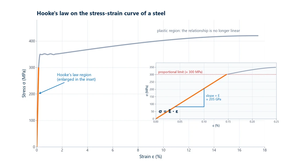
When unloaded after yielding, the metal returns along a straight line parallel to the elastic portion, which shows that elastic behavior still exists even after plastic deformation.

Some materials do not follow Hooke's law in a useful way:

• Rubber and elastomers undergo large elastic deformations, but the relationship is not linear.
• Plastics are viscoelastic: their response depends on time and loading rate. That is why ISO 527-1 measures the modulus of plastics only between 0.05% and 0.25% strain.
• Concrete and cast iron have a nonlinear curve from the start, and an initial, secant or chord modulus is used.
• Composites and wood are anisotropic: the modulus depends on direction, and the law has to be written in tensor form, with more elastic constants.

How Hooke's law is measured in the tensile test

The tensile test is the laboratory version of the spring experiment. The universal testing machine moves the grips apart at a controlled speed, and three instruments work together:

• The load cell measures the force F.
• The extensometer, attached to the parallel length of the specimen, measures the elongation ΔL over the gauge length L₀.
• The software converts these into stress (σ = F/A₀) and strain (ε = ΔL/L₀), plots the curve and fits a straight line to the linear portion to obtain the modulus of elasticity.

The extensometer is essential because the strains involved are tiny. The 0.15% at which the linear portion of steel ends corresponds, over a 50 mm gauge length, to less than 0.08 mm. The 0.05% to 0.25% range of ISO 527-1 for plastics corresponds to 25 to 125 micrometers over 50 mm. The machine's crosshead displacement cannot be used for this: besides the elongation of the specimen, it includes grip seating and the deformation of the machine itself, and a modulus calculated from it comes out well below the real value. Exercise 4 shows the size of this error.

The table lists the standards that govern modulus measurement and instrument verification:

Standard	What it specifies
ABNT NBR ISO 6892-1 / ISO 6892-1	Tensile testing of metals at room temperature (ABNT NBR ISO 6892-1 is its adoption in Brazil); the 2019 ISO version includes a normative annex for determining the modulus of elasticity by linear regression
ASTM E111	Determination of Young's modulus, tangent modulus and chord modulus
ISO 527-1	Tensile properties of plastics, with the modulus measured between 0.05% and 0.25% strain
ASTM E83 and ISO 9513	Verification and classification of extensometers
ABNT NBR ISO 7500-1	Verification of the force-measuring system of testing machines (Brazilian adoption of ISO 7500-1)

The universal testing machines from Biopdi, a Brazilian manufacturer based in São Carlos (SP), Brazil, work with 25 mm and 50 mm extensometers for small strains, such as those of metals, and 150 mm and 250 mm extensometers for the large strains of polymers. The BioLab software plots the stress-strain curve and calculates Young's modulus during the test itself. For metals, sheet and welded joints, the dual-column machine from 5 to 50 kN is the starting point; for polymers and elastomers, the single-column machine from 2 to 10 kN. If your laboratory needs to measure the modulus of elasticity, request a quote.

Hooke's law solved exercises

In all exercises, use g = 9.8 m/s².

Exercise 1: deformation of a spring

A spring with constant k = 250 N/m supports, at rest, a 2.0 kg body. What is the deformation of the spring?

Solution. At equilibrium, the elastic force equals the weight: F = m·g = 2.0 × 9.8 = 19.6 N. By Hooke's law, x = F / k = 19.6 / 250 = 0.0784 m. Answer: 7.84 cm.

Exercise 2: spring constant from an experiment

Masses of 50, 100, 150 and 200 g hung from a spring produced elongations of 2.0, 4.0, 6.0 and 8.0 cm. What is the spring constant, and how much energy does the spring store with 200 g?

Solution. The forces are the weights: 0.49, 0.98, 1.47 and 1.96 N. The ratio F/x is the same at every point, so the points lie on a straight line through the origin. Using the last point: k = 1.96 / 0.080 = 24.5 N/m. The energy is E_p = ½ × 24.5 × (0.080)² = 0.0784 J.

Exercise 3: springs in series and in parallel

Two springs, with k₁ = 200 N/m and k₂ = 300 N/m, receive a force of 60 N. What is the deformation of the assembly in series and in parallel?

Solution. In series: k_eq = (200 × 300) / (200 + 300) = 120 N/m, and x = 60 / 120 = 0.50 m. In parallel: k_eq = 200 + 300 = 500 N/m, and x = 60 / 500 = 0.12 m. The parallel assembly is four times stiffer than the series one.

Exercise 4: modulus of elasticity in a tensile test

A cylindrical steel specimen with a 10 mm diameter is pulled in tension with an extensometer of 50 mm gauge length. In the linear portion, the force goes from 4.0 kN to 12.0 kN, and the extensometer records elongations of 0.0127 mm and 0.0382 mm. What is the modulus of elasticity?

Solution. Area: A₀ = π × 5² = 78.54 mm². Change in stress: Δσ = 8,000 N / 78.54 mm² = 101.9 MPa. Change in strain: Δε = (0.0382 − 0.0127) / 50 = 0.000510. Modulus: E = Δσ / Δε = 101.9 / 0.000510 ≈ 199,700 MPa. Answer: E ≈ 200 GPa, the expected value for a steel. The highest stress in the range, 12,000 / 78.54 = 153 MPa, is below the yield strength of an annealed 1020 steel (about 180 MPa), which confirms that the calculation was made within the Hooke's law regime.

If the same calculation used the machine's crosshead displacement instead of the extensometer, for example 0.10 mm over this range, the apparent strain would be 0.10 / 50 = 0.002 and the modulus would come out at about 51 GPa, four times lower than the real value. This is the error described in the section on the tensile test, and the reason the modulus is measured with an extensometer.

Exercise 5: elongation of an aluminum bar

An aluminum bar (E = 69 GPa), 2.0 m long with a 100 mm² cross section, receives a tensile force of 3.0 kN. How much does it elongate?

Solution. Stress: σ = 3,000 / 100 = 30 MPa, below the yield strength of annealed aluminum (about 35 MPa), so Hooke's law applies. Bar stiffness: k = E·A / L = 69,000 N/mm² × 100 mm² / 2,000 mm = 3,450 N/mm. Elongation: δ = F / k = 3,000 / 3,450 = 0.87 mm. The bar behaves like a very stiff spring.

Exercise 6: generalized Hooke's law in a steel block under biaxial stress

A 100 × 50 × 20 mm steel block receives σ_x = +120 MPa (tension) in the 100 mm direction and σ_y = −60 MPa (compression) in the 50 mm direction, with σ_z = 0 through the 20 mm thickness. With E = 200 GPa and ν = 0.3, the values given in NBR 8800 (the Brazilian standard for the design of steel structures), calculate the change in the three dimensions and in volume.

1. Regime: 120 MPa and 60 MPa are below the minimum yield strength of A36 steel, 250 MPa, so Hooke's law applies.
2. ε_x = [120 − 0.3 × (−60 + 0)]/200,000 = 138/200,000 = 6.90 × 10⁻⁴, and Δa = 6.90 × 10⁻⁴ × 100 = +0.069 mm.
3. ε_y = [−60 − 0.3 × (120 + 0)]/200,000 = −96/200,000 = −4.80 × 10⁻⁴, and Δb = −4.80 × 10⁻⁴ × 50 = −0.024 mm.
4. ε_z = [0 − 0.3 × (120 − 60)]/200,000 = −18/200,000 = −9.0 × 10⁻⁵, and Δt = −9.0 × 10⁻⁵ × 20 = −0.0018 mm. The thickness changes with no stress in z: this is the plane stress state.
5. Volume: ε_V = (6.90 − 4.80 − 0.90) × 10⁻⁴ = 1.20 × 10⁻⁴. By the direct formula, (1 − 0.6)/200,000 × (120 − 60 + 0) = 0.4 × 60/200,000 = 1.20 × 10⁻⁴, the same value. With V = 100,000 mm³, ΔV = +12 mm³.

With σ = E·ε applied only in x, the strain would come out at 120/200,000 = 6.0 × 10⁻⁴, 13% below the real value of 6.9 × 10⁻⁴. The difference is the compression in y, which elongates the block in x through the Poisson effect.

Exercise 7: polymer confined in a rigid die

A rigid polymer block 50 mm high, with E = 2.0 GPa and ν = 0.40, is compressed with σ_z = −10 MPa inside a rigid die that prevents lateral deformation (ε_x = ε_y = 0). The values fall within the ranges given on this site: polypropylene from 1.1 to 2 GPa in this article, and rigid polymers from 0.33 to 0.40 in the article on Poisson's ratio. Calculate the lateral stress and the shortening, and compare with the free block.

1. From ε_x = 0: σ_x − ν(σ_y + σ_z) = 0. By symmetry, σ_x = σ_y, so σ_x = ν/(1 − ν)·σ_z = 0.4/0.6 × (−10) = −6.67 MPa: the die squeezes the block laterally.
2. ε_z = [σ_z − ν(σ_x + σ_y)]/E = [−10 − 0.4 × (−13.33)]/2,000 = −4.667/2,000 = −2.33 × 10⁻³, and Δh = −2.33 × 10⁻³ × 50 = −0.117 mm.
3. Free block: ε_z = −10/2,000 = −5.0 × 10⁻³, and Δh = −0.25 mm.
4. Constrained modulus: M = 2,000 × 0.6/(1.4 × 0.2) = 1,200/0.28 = 4,286 MPa, or 2.14·E. Check: 5.0/2.333 = 2.14.

The same material appears twice as stiff when confined, as the M/E table predicts. For a real polymer, the result is an estimate for rapid loading, because the response of plastics depends on time, as explained in the section on the limits of the law.

References

• HOOKE, R. Lectures de Potentia Restitutiva, or of Spring Explaining the Power of Springing Bodies. London: John Martyn, 1678.
• HOOKE, R. A Description of Helioscopes, and Some Other Instruments. London, 1676.
• YOUNG, T. A Course of Lectures on Natural Philosophy and the Mechanical Arts. London, 1807.
• CALLISTER, W. D.; RETHWISCH, D. G. Materials Science and Engineering: An Introduction. Wiley. Tables 6.1 and 6.2.
• ISO 6892-1:2019. Metallic materials: Tensile testing, Part 1: Method of test at room temperature.
• ISO 527-1:2019. Plastics: Determination of tensile properties, Part 1: General principles.
• ASTM E111. Standard Test Method for Young's Modulus, Tangent Modulus, and Chord Modulus.
• ASTM E83-25. Standard Practice for Verification and Classification of Extensometer Systems.
• LORD, J. D.; MORRELL, R. M. Elastic modulus measurement: obtaining reliable data from the tensile test. Metrologia, vol. 47, no. 2, S41, 2010. DOI: 10.1088/0026-1394/47/2/S05.
• ABNT NBR 6118. Projeto de estruturas de concreto [Design of concrete structures; Brazilian standard].
• CURY, A. Lei de Hooke generalizada [Generalized Hooke's law]. Resistência dos Materiais 2 (MAC003), lecture slides. Juiz de Fora: UFJF, 2026.
• BUFFONI, S. Resistência dos Materiais, aula 7: lei de Hooke generalizada [Strength of Materials, lecture 7: generalized Hooke's law]. Niterói: UFF.
• IAG-USP. AGG0305: 3. Constantes elásticas e Lei de Hooke [Elastic constants and Hooke's law]. São Paulo: Institute of Astronomy, Geophysics and Atmospheric Sciences, University of São Paulo (USP), 2014.
• NEMETH, M. P. An In-Depth Tutorial on Constitutive Equations for Elastic Anisotropic Materials. NASA/TM-2011-217314. Hampton: NASA Langley Research Center, 2011.