
A fatigue test applies a controlled cyclic load to a test specimen until it fractures, or until it reaches a set number of cycles (usually 107), to measure how many cycles the material withstands at each stress level. The result is the S-N curve, or Wöhler curve. From it you get the fatigue limit (steels) or the fatigue strength at a given number of cycles (aluminum and copper). The core standards for metals are ISO 1099:2017 and ASTM E466-21 (axial loading), ISO 1143:2021 (rotating bending) and ASTM E606 (low-cycle fatigue, under strain control).
Fatigue is how shafts, springs, connecting rods, bolts, welds and implants fail: they fracture at stresses well below their static strength, after millions of cycles. This guide covers how a fatigue crack forms and grows, the cycle parameters, the types of fatigue test, the S-N curve, the procedure, the effect of mean stress, how to correct specimen data for a real part, Miner's rule, and how each family of materials behaves. It also includes worked examples, a calculator and the current standards.
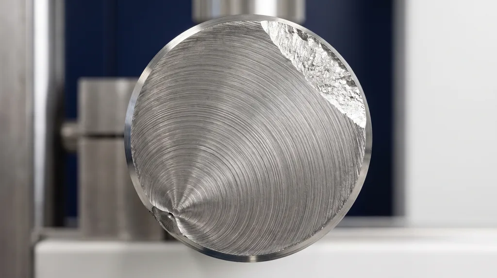
The photo shows the fracture surface of a steel shaft that failed by fatigue. The crack started at the edge and grew slowly, leaving curved lines that are concentric around the origin. The rough region on the opposite side is what was left of the cross-section when it could no longer carry the load and broke all at once. Each of these regions is explained below.
What is a fatigue test
In engineering, fatigue is progressive, localized damage caused by repeated loading. A crack forms and grows a little with each cycle, at stresses below the yield strength, until the remaining cross-section can no longer carry the load and the part fractures suddenly. ASTM E1823 sets out the fatigue and fracture terminology used by the other standards. ISO 1099 describes the axial test under force control. The nominal stress is the force divided by the cross-sectional area (S = F/A), and the goal is to find the relationship between the applied stress and the number of cycles to failure.
The test is needed because a tensile test cannot predict fatigue. A steel with an ultimate tensile strength of 600 MPa can fail at a stress amplitude of 300 MPa after a million cycles. The history of fatigue testing starts with August Wöhler, who studied failures of railway axles in Germany between 1852 and 1869 and gave the curve its name.
The test answers questions that no static test can: how many cycles the material survives at each load level, the amplitude below which it does not fail, and where the crack starts. With these answers you can estimate service life, compare materials, surface finishes and treatments, and validate a component before it goes into service. That is why fatigue testing, one of the most important mechanical tests for design, is routine in industries where loads repeat millions of times: automotive, aerospace, steel structures, electronics and biomedical devices such as prostheses and implants.
Note: "fatigue" is also a health term (physical or mental tiredness). This article covers only the fatigue of materials.
How a fatigue crack forms and grows
Fatigue failure goes through three stages, and each one leaves its own mark on the fracture surface:
- Initiation: the crack starts at a stress concentration: the surface, a notch, an inclusion, a pore or the toe of a weld bead. That is why surface finish has such a strong effect on fatigue life.
- Stable crack growth: the crack grows a little with each cycle. In the intermediate regime the growth rate follows Paris' law, da/dN = C·(ΔK)m, where a is the crack length, N is the number of cycles and ΔK is the stress intensity factor range at the crack tip, with m between 2 and 4 for many metals. ASTM E647-24 measures this curve on precracked specimens.
- Final fracture: when the remaining cross-section can no longer carry the load, the part fails by overload in a rough zone. The larger this zone is compared with the cracked area, the higher the nominal stress was.
The fracture surface tells the story. Beach marks are curved, concentric lines, visible to the naked eye, that spread from the origin and record stops or changes in loading. Striations are microscopic, seen under a scanning electron microscope, and usually each one corresponds to one cycle: a single beach mark can contain thousands of striations. Fractography, with sample preparation by metallography, is what confirms that a part failed by fatigue.
Cycle parameters: amplitude, mean stress and R ratio
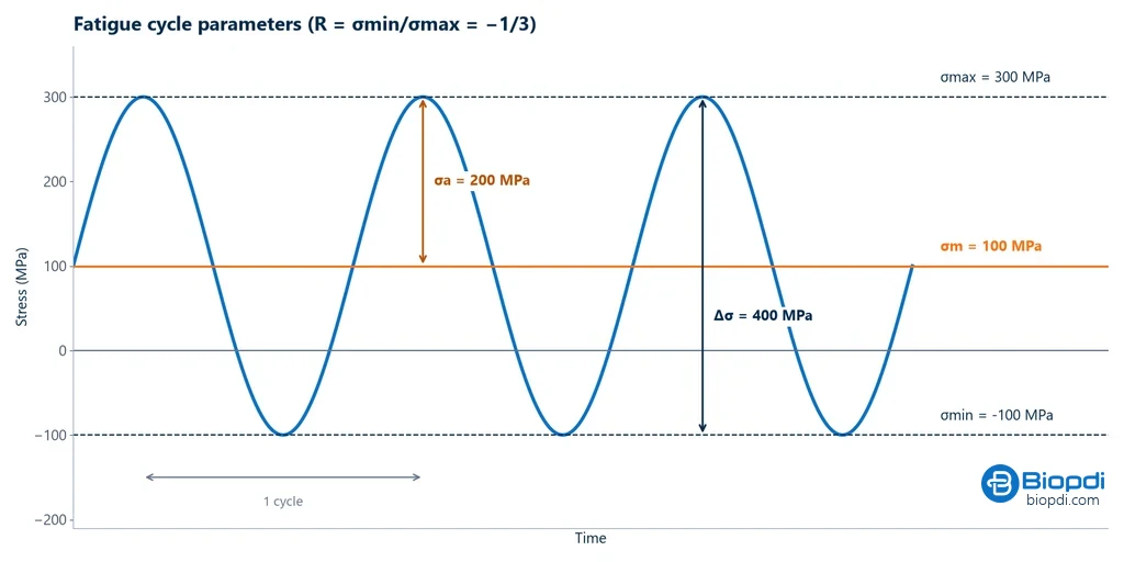
A load cycle is described by a few quantities, all derived from the maximum and minimum stresses. The chart below shows a sinusoidal cycle that goes from 300 MPa in tension to 100 MPa in compression: the mean stress is 100 MPa, the amplitude (half the oscillation) is 200 MPa and the stress range is 400 MPa.
The table lists the formula for each quantity. By convention, tension is positive and compression is negative:
| Quantity | Formula | Note |
|---|---|---|
| Maximum and minimum stress | σmax = Fmax/A0; σmin = Fmin/A0 | compression is negative |
| Mean stress | σm = (σmax + σmin) / 2 | shifts the cycle up or down |
| Amplitude | σa = (σmax − σmin) / 2 | vertical axis of the S-N curve |
| Range | Δσ = σmax − σmin = 2σa | used in crack growth |
| Stress ratio | R = σmin / σmax | R = −1 fully reversed; R = 0 zero-to-tension (pulsating); R = 0.1 common in axial testing |
The R ratio sums up the shape of the cycle in a single number. With R = −1 the cycle is fully reversed: the stress goes from the maximum in tension to the same value in compression, and the mean is zero. With R = 0 it pulses between zero and the maximum. With R = 0.1 the specimen is always in tension, between 10% and 100% of the maximum force. In the cycle shown in the chart, R = −100 / 300 = −0.33.
A fatigue result without the R ratio does not tell you much: the same amplitude with a tensile mean stress gives a shorter life. That is why every S-N curve states the R ratio (or the mean stress) and the type of loading.
Types of fatigue test
The way the load is applied defines the type of test. In an axial test, the cyclic force acts along the specimen axis and the whole gauge section sees the same stress. In rotating bending, a bar rotates under a constant bending moment: each point on the surface goes from tension to compression with every revolution, and the maximum stress is at the surface. The other types cover specific cases: sheets bent in both directions, torsion, strain control for high loads, growth of an existing crack, and testing of the complete part. The table summarizes each one:
| Type | How it loads | Typical R | Standard |
|---|---|---|---|
| Axial (tension and compression) | cyclic force along the specimen axis | −1, 0 or 0.1 | ISO 1099:2017; ASTM E466-21 |
| Rotating bending | bar rotates under a constant bending moment; each revolution is one cycle | −1 | ISO 1143:2021 |
| Plane reversed bending | sheet bent to one side and then the other | variable | depends on the product |
| Torsional | cyclic torque | −1 common | depends on the product |
| Strain control | an extensometer controls the strain | −1 common | ASTM E606-21; ISO 12106:2017 |
| Crack growth | precracked specimen | 0.1 common | ASTM E647-24 |
| Component | the actual part under service loading | depends on the application | e.g., ISO 14801:2016 (dental implant) |
Rotating bending, on an R.R. Moore type machine, is the test that produced the classic fatigue limits of steel, which are used in the estimate in the next section. Dental implant testing under ISO 14801 is an example of a component test: it applies the load at a 30° angle, sinusoidal between the peak and 10% of it (R = 0.1), at up to 15 Hz in air and at most 2 Hz in liquid, up to 5×10⁶ cycles.
S-N curve (Wöhler curve) and fatigue limit
The S-N curve is the main result of the test. Each specimen is tested at a constant amplitude until it fails, and each pair of amplitude and number of cycles becomes a point on the chart: stress amplitude on the vertical axis and cycles to failure on the horizontal axis, on a logarithmic scale, because lives range from a thousand to tens of millions of cycles. The lower the amplitude, the longer the life. The chart below compares the two possible behaviors: steel, whose curve levels off from about one million cycles, and 6061-T6 aluminum, which keeps falling.
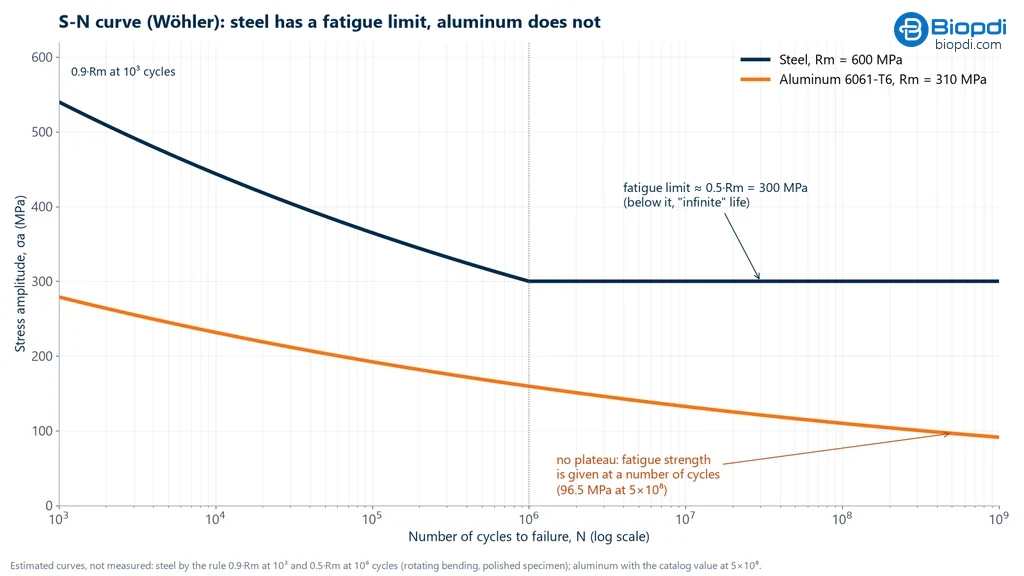
This difference defines the two properties the test delivers. The fatigue limit (endurance limit) is the stress below which the material withstands a very large number of cycles: it is the horizontal plateau seen in steels and titanium alloys. Fatigue strength is the stress that causes failure at a specified number of cycles: it is the figure given for aluminum, copper and magnesium, whose curves never level off, so it always comes with the number of cycles.
For steel, on a polished specimen in rotating bending, the fatigue limit is estimated as S'e ≈ 0.5·Rm, where Rm is the ultimate tensile strength, up to Rm = 1,400 MPa, with a ceiling of about 700 MPa above that (Shigley). Observed values range from 35% to 60% of the ultimate tensile strength.
In high-cycle fatigue, the sloped part of the curve follows Basquin's equation (1910):
σa = σ'f · (2Nf)b
where σ'f is the fatigue strength coefficient, 2Nf is the number of reversals to failure (two per cycle) and the exponent b is typically between −0.05 and −0.12. Without test data, a classic design estimate joins two points with a straight line on the log-log chart: 0.9·Rm at 103 cycles and the fatigue limit at 106 cycles.
The table lists published values. For the titanium alloys, results on notched specimens are also shown. Kt is the theoretical stress concentration factor of the notch: the ratio between the stress at the notch root and the nominal stress.
| Material | Rm | Fatigue limit or fatigue strength | Condition |
|---|---|---|---|
| Cold-drawn SAE 1045 steel | 630 MPa | ≈ 315 MPa (estimated as 0.5·Rm) | rotating bending, 106 cycles |
| 6061-T6 aluminum | ≈ 310 MPa | 96.5 MPa | 5×10⁸ cycles, R = −1 |
| 7075-T6 aluminum | n/a | 159 MPa | 5×10⁸ cycles, R = −1 |
| Annealed Ti-6Al-4V | 950 MPa | 510 MPa smooth; 240 MPa notched (Kt = 3.3) | 107 cycles |
| Solution-treated and aged Ti-6Al-4V | 1,170 MPa | 700 MPa smooth; 160 MPa notched (Kt = 3.3) | 107 cycles |
Sources: Shigley (steel), ASM/MatWeb data sheets (aluminum and titanium). The titanium data make an important point: the condition that is strongest on a smooth specimen (700 MPa) is the most notch-sensitive (it drops to 160 MPa). "Infinite life" is also an engineering convention: very-high-cycle research shows failures below the fatigue limit between 108 and 109 cycles, starting at inclusions below the surface.
Low-cycle, high-cycle and very-high-cycle fatigue
The S-N curve works well for long lives, where the stress stays below yield and the strain in each cycle is elastic. At higher loads, each cycle deforms the material plastically and life drops to thousands of cycles: this is low-cycle fatigue. In this regime the stress changes little while the strain changes a lot, so the test controls strain with an axial extensometer, and the result is the strain-life curve (ε-N), described by the Coffin-Manson relationship. The table compares the two regimes:
| Aspect | High-cycle | Low-cycle |
|---|---|---|
| Life | above about 104 to 105 cycles | below about 105 cycles (ASTM E606) |
| Strain | mostly elastic | plastic in every cycle |
| Test control | force | strain, with an axial extensometer |
| Model | Basquin, S-N curve | Coffin-Manson, ε-N curve |
| Standards | ISO 1099:2017, ASTM E466-21, ISO 1143:2021 | ASTM E606/E606M-21, ISO 12106:2017 |
| Examples | shafts, springs, wheels, bolts | pressure vessels, turbines during startup and shutdown, thermal cycles |
Beyond 108 to 109 cycles is very-high-cycle fatigue, studied on ultrasonic machines at about 20 kHz. These are the three fatigue regimes of materials.
How the fatigue test is performed
The test repeats the same procedure on several test specimens, each at a different stress level, until the S-N curve is built. The result depends as much on specimen preparation as on the machine, because a fatigue crack starts at the surface and at any defect.
Test specimen
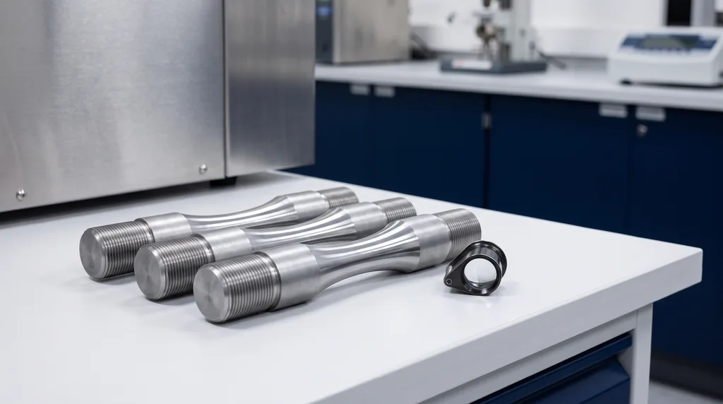
The choice of test specimen depends on the material and the type of loading, and the specimen must represent the conditions of the real part. For metals, the geometry is the one given by the test standard (ISO 1099 or ASTM E466 for axial loading, ISO 1143 for rotating bending): circular or rectangular cross-section, a polished gauge section and a large-radius transition to the ends, so the crack does not start at a machining mark or a corner. In rotating bending, the specimen can be cylindrical, tapered or hourglass-shaped. Polymers, ceramics and composites call for geometries specific to each standard, and when the product itself is what matters, the actual component is tested, such as the implant in ISO 14801. The photo shows steel test specimens for axial fatigue: threaded ends for gripping, a mirror-polished hourglass center section and a continuous transition, with no corner where a crack could start.
Step by step
- Prepare and measure the test specimen: check the finish of the gauge section for scratches and measure the area A0, which converts force into stress.
- Mounting: grips aligned. In axial testing, misalignment adds bending and reduces life.
- Loading: set the amplitude, the R ratio, the waveform (usually sinusoidal) and the frequency.
- End criterion: fracture, loss of a percentage of stiffness or force, or the cycle limit (runout), for example 107.
- Several levels: the test is repeated at several stress levels, with several specimens at each, and the S-N curve is plotted.
What is measured during the test
The load cell measures force at every cycle, and the controller corrects the drive to hold the programmed amplitude; the counter records cycles until the end criterion is reached. As the crack grows, the stiffness of the specimen drops, and this drop serves as a warning or as a stop criterion. Strain is measured with an extensometer attached to the specimen, either a contact type (clip-on) or an electrical gauge bonded to the surface (strain gauge). It is essential in strain control and records the hysteresis loops, the stress-strain curve of each cycle, which show how much energy the material dissipates and whether it hardens or softens with repetition. Optical, non-contact extensometers are used for specimens that are small, hot or cannot take anything clamped to them. Actuator displacement is also recorded, but it includes the clearances of the setup and gives only an indirect measure of strain.
Scatter, statistics and duration
Scatter is large, even under strict control: small differences in chemistry, heat treatment and surface finish change the life. ISO 12107:2012 defines the statistical planning, and the published curve is usually the one for 50% probability of failure. To find the fatigue limit, the staircase method is used (up-and-down, Dixon and Mood, 1948): if the specimen fails before 107 cycles, the next one goes one step lower; if it survives, one step higher.
Time is the main cost of the test: 107 cycles at 100 Hz take about 28 hours per specimen; the 5×10⁶ cycles of ISO 14801 at 15 Hz take almost 4 days, and at 2 Hz in a liquid medium, 29 days. Raising the frequency shortens the test, and for metals in air it has little effect on the result; for polymers and in corrosive media it matters, as the section on materials shows further on.
Mean stress effect: Goodman, Gerber and Soderberg
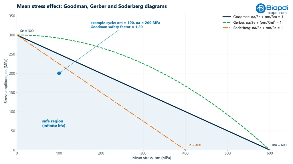
With a tensile mean stress, the allowable amplitude drops, because the tensile part of the cycle, the part that opens the crack and drives it forward, gets larger. The Haigh diagram (amplitude × mean stress) connects the fatigue limit Se (that of the part, corrected as shown in the next section) on the amplitude axis to a strength on the mean stress axis: the ultimate tensile strength Rm or the yield strength Re. The safety factor n comes from one of these three criteria:
- Goodman: σa/Se + σm/Rm = 1/n. A straight line to the ultimate tensile strength, the criterion most used in design.
- Gerber: n·σa/Se + (n·σm/Rm)² = 1. A parabola that fits data for ductile metals better.
- Soderberg: σa/Se + σm/Re = 1/n. A straight line to yield, the most conservative.
The diagram below shows the three curves side by side. A cycle is a point defined by its mean stress and its amplitude: below the chosen curve it is safe, and the closer it is to the curve, the lower the safety factor. The Soderberg line lies inside the others, and the Gerber parabola outside.
A compressive mean stress tends to help: this is the principle of shot peening, which leaves compressive residual stress at the surface and delays crack nucleation. The calculator below does the math for your cycle.
From test specimen to part: Marin factors and notches
The fatigue limit measured on a small, polished specimen in rotating bending (S'e) is higher than that of the real part, which has a different finish, a different size and a different type of loading. The Marin equation corrects the value by multiplying it by one factor for each difference:
Se = ka · kb · kc · kd · ke · S'e
The table shows what each factor corrects and the reference values:
| Factor | Corrects for | Values (Shigley) |
|---|---|---|
| ka | surface finish | ka = a·Rmb: ground a = 1.58 and b = −0.085; machined a = 4.51 and b = −0.265; hot-rolled a = 57.7 and b = −0.718; as-forged a = 272 and b = −0.995 |
| kb | size | bending or torsion: 1.24·d−0.107 (2.79 to 51 mm); axial: 1 |
| kc | type of loading | bending 1; axial 0.85; torsion 0.59 |
| kd | temperature | depends on the material |
| ke | reliability | 0.897 (90%); 0.868 (95%); 0.814 (99%) |
For a steel with Rm = 630 MPa, surface finish alone brings ka to 0.92 (ground), 0.82 (machined), 0.56 (hot-rolled) and 0.45 (as-forged). Notches enter through the fatigue notch factor Kf = 1 + q(Kt − 1), where Kt is the theoretical stress concentration factor and q is the notch sensitivity, between 0 and 1: Kf is always less than or equal to Kt.
The Marin factors do not cover everything. Chemical composition, microstructure, heat treatment and internal defects, such as pores and inclusions, also change fatigue life, and the environment matters a great deal: in a corrosive medium, life drops and steel no longer has a defined plateau.
Cumulative damage: the Palmgren-Miner rule
Real parts do not work at a single amplitude. Miner's rule (1945) adds up the fraction of life consumed at each level:
D = Σ ni / Ni, and failure is predicted when D = 1
where ni is the number of cycles applied at level i and Ni is the life at that level, taken from the S-N curve. It is simple and widely used, but it is linear and ignores load order: high-load blocks followed by low-load blocks tend to fail at D below 1, and the reverse at D above 1. For irregular load histories, cycles are counted with the rainflow method (ASTM E1049).
Fatigue testing by material
The test principle is the same for any material, but the damage mechanism, the precautions during the test and what is sought in the result change from one family to another.
Metals
For metals, the previous sections apply: steels and titanium alloys have a fatigue limit; aluminum, copper and magnesium do not, and are designed for a finite life in cycles. In the automotive industry, springs, shafts and chassis components are tested; in aerospace, the aluminum alloys of wings and fuselages; in steel structures such as bridges, the critical point is the welded joints, where the weld toe concentrates stress. In a corrosive medium, frequency starts to matter: the slower the cycle, the longer the medium acts on the crack tip in each cycle, and the shorter the life in cycles.
Polymers
Polymers are viscoelastic: their response depends on the loading rate and the time under load. Part of the energy of each cycle turns into heat through hysteresis, and since polymers conduct heat poorly, the specimen heats up; at high frequency it can soften and fail from heating, not from a crack. For this reason, frequency and temperature must be controlled and reported with the result. The test also evaluates resistance to crack growth and the degradation of the material over time, in components of sports equipment and machine parts.
Ceramics
Ceramics resist compression well but are brittle: they do not deform plastically to relieve the tip of a crack, and a small defect is enough to initiate failure under cyclic loading. Humidity and ambient temperature accelerate the slow growth of these cracks, so they are part of the test conditions. This is the case for technical ceramics in electronics, in aerospace components and in dental prostheses, evaluated by mechanical cycling.
Composites
In fiber composites, damage is not a single crack: matrix cracks, fiber-matrix debonding and separation between plies (delamination) appear, spread throughout the volume. The result depends on the fiber direction relative to the load, the matrix and the interface between plies, and loss of stiffness is usually the failure criterion before fracture. Tension-tension fatigue testing of polymer matrix composites follows ASTM D3479. It is the test that qualifies composites for aircraft structures, such as wings, and for sports vehicle components.
Solved fatigue exercises
Exercise 1: cycle parameters. Steel test specimen with d = 8.0 mm, tested at Fmax = +15 kN and Fmin = −5 kN.
A0 = π × 8.0² / 4 = 50.27 mm². σmax = 15,000 / 50.27 = 298.4 MPa and σmin = −5,000 / 50.27 = −99.5 MPa. σm = (298.4 − 99.5) / 2 = 99.5 MPa; σa = (298.4 + 99.5) / 2 = 198.9 MPa; R = −99.5 / 298.4 = −0.33.
Exercise 2: life from the Basquin line. Cold-drawn SAE 1045 steel, Rm = 630 MPa, S'e = 0.5 × 630 = 315 MPa at 106 cycles and 0.9 × 630 = 567 MPa at 103 cycles. What is the life at σa = 400 MPa and R = −1?
b = log(315/567) / 3 = −0.0851. N = 103 × (400/567)1/b = 103 × 0.7055−11.75 ≈ 6.0 × 10⁴ cycles.
Exercise 3: Marin and Goodman on a machined shaft. Same steel (Rm = 630 MPa, Re = 530 MPa), 25 mm machined shaft in rotating bending, with σa = 100 MPa and σm = 150 MPa.
ka = 4.51 × 630−0.265 = 0.817; kb = 1.24 × 25−0.107 = 0.879; Se = 0.817 × 0.879 × 315 = 226 MPa. Goodman: 1/n = 100/226 + 150/630 = 0.680, so n = 1.47. Soderberg: 1/n = 100/226 + 150/530 = 0.725, so n = 1.38. The limit of the polished specimen dropped 28% in the real part.
Exercise 4: cumulative damage. Using the curve from exercise 2, the part undergoes 10,000 cycles at 400 MPa and 100,000 cycles at 350 MPa. How many more cycles can it withstand at 380 MPa?
N(400) = 60,360, D1 = 0.166. N(350) = 289,900, D2 = 0.345. Remaining: 1 − 0.166 − 0.345 = 0.489. N(380) = 110,300, so n3 = 0.489 × 110,300 ≈ 54,000 cycles, with the caveat that Miner ignores the order of the blocks.
Exercise 5: how long the test takes. 107 cycles at 100 Hz = 105 s ≈ 27.8 h. On a cycling machine at 5 Hz, 5×10⁶ cycles = 106 s ≈ 11.6 days per batch; with several samples at the same time, the time per sample drops in the same proportion.
Common mistakes in fatigue testing
- Assuming every material has a fatigue limit. Aluminum, copper and magnesium do not: the fatigue strength at a given number of cycles is used instead.
- Saying titanium has no limit. Titanium alloys have a plateau, like steels.
- Using 0.5·Rm directly in design. It applies to a polished specimen; for the part, apply the Marin factors (in exercise 3, from 315 to 226 MPa).
- Applying 0.5·Rm above 1,400 MPa. Above that, the ceiling is about 700 MPa.
- Confusing σa with σmax or Δσ. Always state which quantity is on the axis and what R is.
- Ignoring mean stress. The same amplitude with a different R gives a different life.
- Treating Kt as Kf. In fatigue, Kf = 1 + q(Kt − 1), less than or equal to Kt.
- Extrapolating the curve beyond the tested range, such as estimating 109 cycles from data up to 107.
- Citing ASTM E739 as current (it was withdrawn in 2024) or ASTM E8 as a fatigue standard (it is a tensile standard).
- Ignoring frequency for polymers and in corrosive media.
- Confusing beach marks with striations, or fatigue with creep, which is deformation under constant load at high temperature.
- Taking Miner's rule as exact. It is a linear approximation, sensitive to the load sequence.
Fatigue testing standards
The standard depends on the material, the type of loading and the regime. For metals, the basic ones are ISO 1099 and ASTM E466 for axial testing, ISO 1143 for rotating bending, and ASTM E606 and ISO 12106 for low-cycle fatigue; composites and products, such as implants, have their own standards. The table lists the most widely used:
| Standard | Subject |
|---|---|
| ASTM E1823-26a | terminology for fatigue and fracture testing |
| ISO 1099:2017 | axial force-controlled fatigue, constant amplitude |
| ASTM E466-21 | axial force-controlled fatigue, predominantly elastic regime |
| ISO 1143:2021 | rotating bending fatigue |
| ASTM E606/E606M-21 | strain-controlled fatigue (low cycle) |
| ISO 12106:2017 | axial strain-controlled fatigue |
| ISO 12107:2012 | statistical planning and analysis of fatigue data |
| ASTM E647-24 | fatigue crack growth rate (da/dN × ΔK) |
| ASTM D3479 | tension-tension fatigue of polymer matrix composites |
| ISO 14801:2016 | dynamic loading test for dental implants |
Fatigue testing machine
Every fatigue testing machine has the same three parts: a drive system, which applies the cyclic load; a measurement system, with a load cell and, when needed, an extensometer; and a control and data acquisition system, which holds the amplitude, counts the cycles and records force, strain and frequency. What changes is the speed. High-cycle fatigue calls for fast machines: servo-hydraulic, resonant (which run at tens to hundreds of hertz), rotating bending (up to thousands of revolutions per minute) and, in the very high cycle range, ultrasonic machines at 20 kHz. A slow machine would take months to reach 107 cycles.
The panel below shows the universal testing machine and the role of each of its parts in a cyclic test:
The universal testing machine in fatigue testing
The M2 line has single-column models, from 200 N to 10 kN, and dual-column models, from 5 kN to 1,000 kN. Each part of the machine has a role in the test:
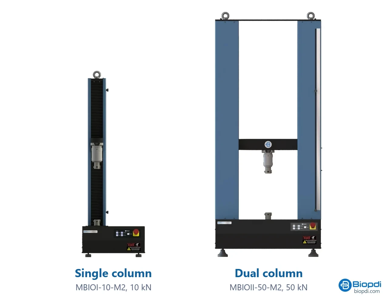
- Moving crosshead repeated loading and unloading steps
- Load cell measures the force in each cycle
- Grips or fixture the same as for tension, compression or bending
- Extensometer hysteresis loops
- BioLab software step-based cyclic tests
- Control panel and emergency stop positions and stops the test
At Biopdi, mechanical cycling performs fatigue tests with load and frequency control for dentistry and biomaterials: the Biocycle cycling machine tests several specimens at the same time (2 to 12, depending on the model), with a load of 0 to 2,000 N per specimen, pneumatic pistons of up to 5 Hz, cycle counting up to 1 trillion cycles with automatic stop, and an optional sliding module to simulate bruxism. For simultaneous thermal and mechanical cycles, there is thermomechanical cycling.
The universal testing machine performs step-based cyclic tests, with constant or variable force programmed in the BioLab software: loading and unloading, hysteresis loops and low-count cycling. It can also be fitted with a dynamic module for fatigue testing; frequency and load range depend on the configuration, available on request. It also measures the tensile strength and yield strength that feed the Goodman and Marin estimates. For non-standard setups, see our special projects or request a quote.
Other tests and technical references
Tests performed on the Biopdi universal testing machine

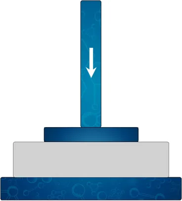
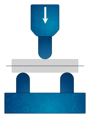

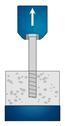


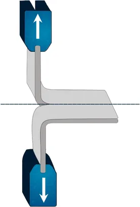



Related technical references
NBR 5739 concrete compression test: fc calculation and the NBR 7222, NBR 12142 and NBR 6136-2 standards
ABNT NBR 5739:2018 (the Brazilian standard for concrete compression testing), reaffirmed in 2023, covers compression testing of cylindrical concrete specimens: continuous loading at 0.45 ± 0.15 MPa/s until failure and fc = 4F/(πD²), in MPa, to three significant figures. See what it requires of the machine and the specimen, the h/d correction, failure types A to G and the related standards: NBR 7222 (splitting tensile test), NBR 12142 (flexural tensile strength) and NBR 12118, withdrawn in February 2026 and replaced by NBR 6136-2:2026.
Crush test: ECT, FCT, RCT and BCT
The crush test compresses corrugated board until it collapses. See ECT, FCT, RCT, CMT and BCT, formulas, McKee, 32 ECT in kN/m, standards and examples.
Compression test: what it is, how to calculate it, concrete (NBR 5739 and fck) and standards
A compression test shortens a specimen until it fractures or yields. Learn to calculate compressive strength, plus NBR 5739, concrete fck and standards.
Frequently asked questions
What is a fatigue test?
It is a test that applies a controlled cyclic load to a test specimen or part until fracture or until a defined number of cycles, such as 107. It is used to build the S-N curve and obtain the fatigue limit or fatigue strength (ISO 1099, ASTM E466).
How do you evaluate the fatigue of a material?
By testing several specimens at different stress levels, counting the cycles to failure and plotting the amplitude against the logarithm of the cycles. Because the scatter is large, ISO 12107 defines the statistical treatment, and the staircase method estimates the fatigue limit.
What are the 3 types of material fatigue?
Low-cycle fatigue (fewer than about 105 cycles, with plastic deformation), high-cycle fatigue (elastic deformation, up to about 107 cycles) and very high cycle fatigue (above 108 to 109 cycles).
What is the S-N curve or Wöhler curve?
It is the plot of stress amplitude (S) against the number of cycles to failure (N, on a logarithmic scale). It is named after August Wöhler, who studied railway axles between 1852 and 1869.
What is the difference between fatigue limit and fatigue strength?
The fatigue limit is the stress below which the material withstands a very large number of cycles, the plateau seen in steels and titanium. Fatigue strength is the stress that causes failure at a specified number of cycles, used for aluminum and copper.
What is the fatigue limit of steel?
For a polished specimen in rotating bending, about 0.5 times the tensile strength, up to 1,400 MPa of tensile strength, and about 700 MPa above that. In the real part it drops with surface finish, size and notches.
Does aluminum have a fatigue limit?
No. The curve keeps falling, so the strength at a fixed number of cycles is reported: 96.5 MPa for 6061-T6 and 159 MPa for 7075-T6, both at 5×10⁸ cycles.
What is low-cycle fatigue?
It is failure in few cycles, below about 105, with plastic deformation in every cycle. It is tested under strain control (ASTM E606, ISO 12106) and described by the Coffin-Manson relation.
What is the Goodman diagram used for?
To correct for the effect of mean stress. The line connects the fatigue limit, on the amplitude axis, to the tensile strength, on the mean stress axis, and the safety factor comes from σa/Se + σm/Rm = 1/n.
What does Miner's rule state?
That each block of cycles consumes a fraction of the life equal to n/N, and failure is predicted when the sum reaches 1. It is simple and widely used, but it ignores the load sequence.
How do you identify a fatigue fracture?
The surface shows the origin at an edge or defect, concentric beach marks visible to the naked eye, microscopic striations and a rough final overload zone.
What machine is used for fatigue testing?
For high-cycle fatigue, servo-hydraulic, resonant and rotating bending machines; for very high cycle fatigue, ultrasonic machines. For dental products, cycling machines such as the Biopdi Biocycle, which tests several specimens at the same time at up to 5 Hz.
Interactive simulation
Try the test in your browser and watch the results being calculated.