
The consolidation test, or oedometer test, determines the consolidation properties of a soil, expressed by the rate and magnitude of its deformation when it is laterally confined, loaded vertically and drained, as defined by ABNT NBR 16853:2020 (the Brazilian standard for one-dimensional consolidation testing). In practice, the test specimen, usually saturated, sits in a rigid ring, drained at both faces, and receives load increments that double at each stage and usually last 24 hours, to measure how much the soil settles and how fast. The compression curve gives the compression index Cc, the recompression index Cr and the preconsolidation stress σ'vm; the height readings over time give the coefficient of consolidation cv. NBR 16853:2020 (Soil: one-dimensional consolidation test) absorbed the technical content of NBR 12007, withdrawn on July 20, 2015, and is still in force, a status checked on October 1, 2026.
In one line: Cc = Δe / Δlog σ' on the virgin compression branch, and cv = 0.848 · Hd² / t90 by Taylor's method. This guide explains Terzaghi's theory in laboratory language, the standards (NBR 16853, ASTM D2435, ASTM D4186 and DNER-IE 005/94), the equipment, the step-by-step procedure, the calculations and the interpretation of the curves, with a worked example that goes from the dial gauge reading to the settlement of a clay layer in the field.
What the consolidation test is and what it is used for
The consolidation test reproduces, on a small sample, the process that makes an embankment settle, a foundation sink and a pavement become wavy over soft clay, in order to predict what will happen to the whole layer. In sand, water leaves the pores almost immediately; in clay, permeability is so low that the same process takes months or years.
What is soil consolidation and consolidation settlement?
Soil consolidation is the slow reduction in volume of a saturated soil as water drains from its pores under sustained load: the load is transferred from the water to the grains and the surface goes down. This lowering is consolidation settlement, which in soft clays takes months or years.
Terzaghi's model, the cylinder with a spring and water detailed in the next section, describes the process in four steps:
- The water takes the load: at the moment of loading, the pore water, practically incompressible, carries the entire increment as excess pore pressure, and the grains do not feel anything yet.
- The water drains: the excess pore pressure pushes the water toward the draining faces, slowly in clay, quickly in sand.
- The grains take the load: as pore pressure drops, effective stress increases, the soil skeleton compresses and the layer settles.
- Equilibrium: once the excess pore pressure has dissipated, the whole load is on the grains and primary consolidation ends; only secondary compression remains, which is much slower.
What questions does the test answer, and what names does it go by?
The consolidation test answers two questions that are often confused in design: how much the structure will settle and how long it will take. The first depends on the compressibility of the soil, measured by Cc, Cr and σ'vm. The second depends on how fast the water can escape, measured by cv. The same test provides both answers, which is why it is required in any study of an embankment or foundation on compressible clay: building foundations, highway and railway embankments, dams, ports, industrial yards and logistics warehouses with heavily loaded floors, and residential developments on coastal lowlands. It is one of the most common laboratory tests in the routine of geotechnical civil engineering.
The two names refer to the same test. "Oedometer" comes from the oedometer (edômetro in Brazilian Portuguese, edómetro in Portugal), the cell with a rigid ring that prevents lateral deformation; "one-dimensional consolidation" is the technical name used by NBR 16853. The literature and test reports also use oedometric compression, confined compression, oedometric test, consolidation test and laterally confined consolidation, all for the same procedure. The diagram below shows the cell in cross-section: the specimen sits inside the ring, between two porous stones, and the load enters through the loading cap while water drains from the top and the bottom.
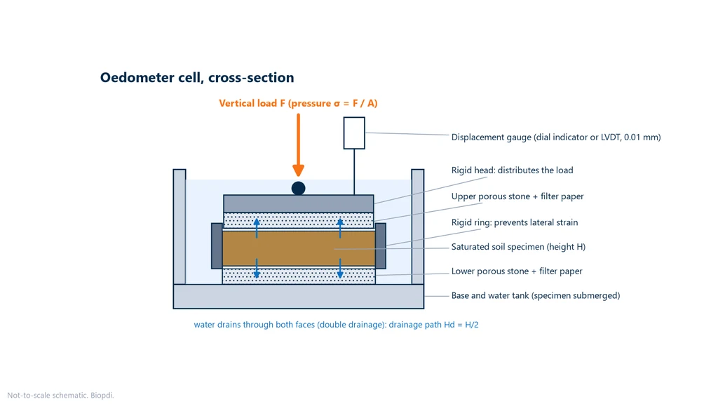
Lateral confinement is what makes the test representative. An extensive clay layer loaded by a wide embankment has nowhere to move sideways: it only compresses vertically. The ring imposes the same condition on the sample, so the deformation measured in the laboratory converts directly into settlement in the field. This is also the difference from the unconfined compression test, in which the specimen is free to expand laterally and fails.
Terzaghi's consolidation theory
The theory behind the test is Karl Terzaghi's one-dimensional consolidation theory, published in 1925. The classic image is a spring inside a cylinder full of water, with a perforated lid. When the load is applied, the water has not yet had time to escape and takes the entire stress increment as excess pore pressure; the spring, which represents the soil skeleton, has not felt anything yet. As the water flows out through the hole, pore pressure drops, the spring starts carrying the load and the assembly shortens.
Soil behaves the same way. The total applied stress is shared between the water and the grains, and only the part that reaches the grains, the effective stress σ', deforms the soil. Settlement follows the dissipation of pore pressure, and the rate of this dissipation is governed by the time factor:
Tv = cv · t / Hd²
Here cv is the coefficient of consolidation, t is time and Hd is the drainage path length, that is, the longest path a drop of water travels to leave the layer. In the oedometer, with a porous stone at the top and bottom, drainage is double and Hd equals half the specimen height. Since time grows with the square of Hd, a 2 cm sample consolidates in minutes what a 6 m layer takes years to consolidate, and it is this proportion that allows the laboratory result to be carried over to the field.
The theory starts from simple assumptions: saturated and homogeneous soil, incompressible water and grains, water flow obeying Darcy's law, and deformation and flow only in the vertical direction. The last two are exactly the ones the oedometer imposes on the sample, with the rigid ring at the sides and the porous stones at the top and bottom.
Terzaghi's solution relates Tv to the degree of consolidation U, the fraction of primary settlement already completed. Two points of this relationship appear in every calculation: U = 50% corresponds to Tv = 0.197 and U = 90% to Tv = 0.848. For intermediate values, the approximations Tv = (π/4)·U² up to U = 60% and Tv = 1.781 − 0.933·log(100 − U%) above that apply.
Once pore pressure has dissipated, the soil still keeps compressing slowly, through rearrangement and creep of the skeleton: this is secondary compression. It appears as a final straight segment on the plot of height versus log time, and its slope is the coefficient Cα. Terzaghi's theory describes only primary consolidation, and NBR 16853 only allows cv to be calculated when the shape of the curve indicates that this theory applies.
Consolidation test standards: NBR 16853, DNER-IE 005/94 and ASTM D2435
In Brazil, the test follows ABNT NBR 16853:2020 (Soil: one-dimensional consolidation test), published in May 2020 and confirmed by ABNT (the Brazilian standards body) in January 2025. It defines the apparatus, specimen preparation, load increments, reading times, calculations (void ratio, cv by Casagrande or Taylor, Cc and σ'vm, the latter by Casagrande or by Pacheco Silva) and the content of the report. The former NBR 12007 was withdrawn on July 20, 2015, NBR 16853 absorbed its technical content, and its procedure should no longer be used as a reference, even though it is still one of the first results when searching for the test online.
For highway projects, DNIT (Brazil's federal transportation infrastructure agency) maintains DNER-IE 005/94 (Soils: consolidation), whose text is publicly available on the gov.br portal. It uses the same logic of doubled load increments and the same reading times, indicates the usual sequence of 20, 40, 80, 160, 320 and 640 kPa (or 25 to 800 kPa), rings with a usual diameter between 63.5 and 107.95 mm, and a height three to four times smaller than the diameter.
Outside Brazil, the reference is ASTM D2435/D2435M, currently in the D2435/D2435M-25 edition, which replaced -11(2020). It has two methods: in method A, each increment lasts 24 hours and time readings are taken in at least two increments; in method B, readings are taken in every increment and each new increment is applied at the end of primary consolidation, which makes it possible to obtain cv and the rate of secondary compression. For the constant rate of strain (CRS) test, ASTM D4186/D4186M applies, in the -20e2 edition. The table summarizes the current editions, checked on October 1, 2026 in the Target catalog for the ABNT standards, on the DNIT portal and in the ASTM store:
| Standard | Subject | Edition and status |
|---|---|---|
| ABNT NBR 16853 | One-dimensional consolidation (incremental) | 2020, in force, confirmed in 01/2025 |
| ABNT NBR 12007 | One-dimensional consolidation (former text) | Withdrawn in 2015 |
| DNER-IE 005/94 | Soils: consolidation (highway) | 1994, published by DNIT |
| ABNT NBR 6457 | Sample preparation and moisture content | 2024, in force |
| ASTM D2435/D2435M | Incremental consolidation, methods A and B | D2435/D2435M-25, active |
| ASTM D4186/D4186M | Controlled-strain consolidation (CRS) | D4186/D4186M-20e2, active |
The three incremental test standards follow the same logic, but differ in details that change the test report. The table compares the main points, with the NBR 16853 clause in parentheses; the ASTM D2435-25 column includes only what appears in the scope published in the ASTM store:
| Item | NBR 16853:2020 | DNER-IE 005/94 | ASTM D2435/D2435M-25 |
|---|---|---|---|
| Load increments | Seating load of 5 or 2 kPa (6.5.1); then about 10, 20, 40 kPa and so on, up to the virgin compression range (6.5.2) | 20, 40, 80, 160, 320 and 640 kPa, or 25 to 800 kPa | Incremental; method A with 24 h increments, method B with a new increment at the end of primary consolidation |
| Ring | Ø ≥ 50 mm (pref. 100), H ≥ 13 mm, D/H ≥ 2.5 (pref. 3.0), diameter variation ≤ 0.03%; no floating ring in very soft soil (4.3) | Usual Ø of 63.5 to 107.95 mm, D/H of 3 to 4; no floating ring in very soft soil | See the standard |
| Loading frame | Accuracy of 0.5% of the applied load; increment applied within 2 s, without impact (4.1) | No equivalent requirement | See the standard |
| Inundation | Right after the 10 kPa increment, for samples saturated in the field or taken below the water table (6.5.3) | Before the first increment | See the standard |
| Readings | 1/8 min to 24 h, including the 30 min reading (6.5.4) | Same series, without the 30 min reading | Method A: time readings in at least 2 increments; method B: in all of them |
| Unloading | At least 3 stages (6.5.6) | Only if the swelling needs to be known | See the standard |
| cv | Casagrande or Taylor, in at least 2 increments, 1 above σ'vm, only if the curve follows Terzaghi (7.4) | Casagrande and Taylor | Method A: in at least 2 increments |
| σ'vm | Casagrande or Pacheco Silva (7.6) | Casagrande | See the standard |
Equipment and test specimen
The setup has three parts: the oedometer cell, which confines and drains the sample; the load frame, which applies and holds the load of each stage; and the displacement gauge, which records the change in height. Under ABNT NBR 16853 (the Brazilian standard for the one-dimensional consolidation test), each part has its own requirements:
- Ring (4.3): minimum inside diameter of 50 mm (100 mm preferred), minimum height of 13 mm and at least 10 times the largest particle, and a diameter-to-height ratio of at least 2.5 (3.0 preferred). For tube samples, the ring diameter must be at least 5 mm (preferably 10 mm) smaller than the tube, so that trimming removes the disturbed edge. The ring must be rigid: under a pressure equal to the maximum test pressure, its diameter may not change by more than 0.03%. The material must not corrode. The usual choice is stainless steel with a well-polished inner face, or a face coated with a low-friction material such as PTFE, to reduce side friction, and the standard recommends greasing the ring with silicone grease. DNER-IE 005/94 (a Brazilian highway agency test method) advises against rings smaller than 63.5 mm in diameter, because the smaller the specimen, the more edge disturbance affects the result.
- Porous stones (4.4): the top stone is 0.2 to 0.5 mm smaller in diameter than the ring, so it moves down with the sample without binding on the wall; with a floating ring, the bottom stone is too. They are separated from the soil by filter paper when needed. For saturated soil, the stones are boiled and kept submerged until assembly; for partially saturated soil, they are only moistened; for expansive, collapsible or very dry soil, they are placed dry (6.4.2).
- Load frame (4.1): applies and holds each load to within 0.5% of the applied value, and transfers each load increment in no more than 2 seconds, without significant impact.
- Displacement gauge (4.7): dial gauge (also called a deflectometer or extensometer in the soil laboratory) or electronic transducer with a resolution of 0.01 mm; the standard calls for a travel of up to 15 mm for the dial gauge.
- Balance (4.6): resolution of 0.01 g, used to weigh the specimen.
The oedometer cell comes in two configurations. In the fixed-ring cell, the ring is clamped to the base and the specimen moves only downward; it is the only one that allows a graduated standpipe to be connected to the bottom porous stone to measure permeability by the falling-head method at the end of a stage. In the floating-ring cell, the ring is free and the sample compresses from both faces, which halves the effect of side friction on the wall. For cv, Cc and σ'vm, both configurations are accepted by NBR 16853, ASTM D2435 and DNER-IE 005/94, but NBR 16853 and the DNER method exclude the floating ring for very soft soil.
The test specimen comes from an undisturbed sample, either a thin-walled (Shelby) tube or a block, and is trimmed directly into the ring, preferably in a humid room so it does not lose moisture. For tube samples, the ends of the tube are discarded. The standard also accepts a laboratory-compacted specimen, provided the report describes how it was prepared. The trimmings give the initial moisture content; the specific gravity of the soil solids comes from a representative portion of the same sample, according to ABNT NBR 6458:2016 (corrected version 2:2017). Both go into the calculation of the void ratio.
There are two ways to apply the load. In the manual frame, a lever type known as the Bishop consolidation press, a lever multiplies the weight of slotted weights placed on a hanger, and displacement is read on a dial gauge. In the automatic electric frame, an actuator applies the load, a load cell measures it and an LVDT records the height. The images below show the two Biopdi consolidation press models, with the parts of each one labeled:
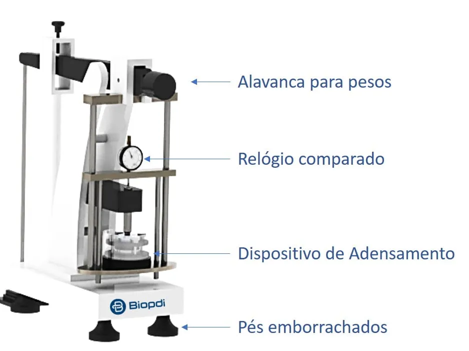
Manual consolidation press: lever, weights and dial gauge
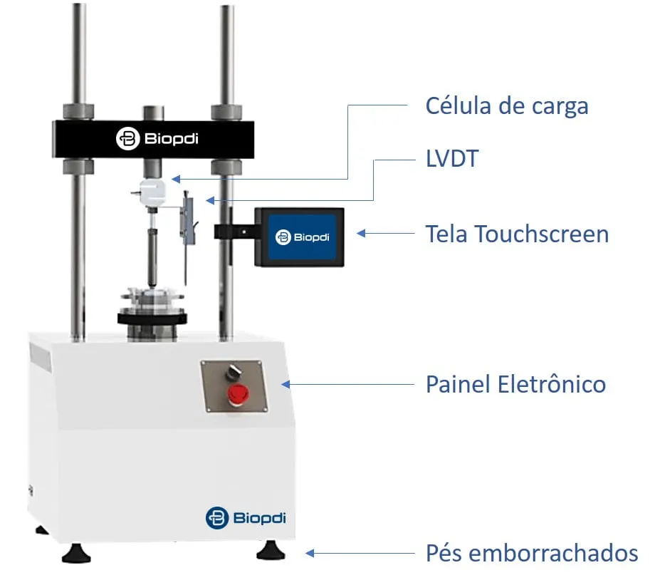
Automatic electric consolidation press: load cell, LVDT and touchscreen
One thing that surprises people coming from metals testing is how small the forces are. The force on the sample is the stage pressure times the ring area (F = σ · A), and even at the high stages it stays at a few kilonewtons. The table shows the force for three ring diameters:
| Pressure (kPa) | Ring Ø 50 mm (19.63 cm²) | Ring Ø 63.5 mm (31.67 cm²) | Ring Ø 100 mm (78.54 cm²) |
|---|---|---|---|
| 10 | 0.020 kN (20 N) | 0.032 kN (32 N) | 0.079 kN (79 N) |
| 160 | 0.314 kN | 0.507 kN | 1.257 kN |
| 640 | 1.257 kN | 2.027 kN | 5.027 kN |
| 1,280 | 2.513 kN | 4.054 kN | 10.05 kN |
In practice, this means that measurement in the low range matters as much as the maximum capacity. A 10 kPa stage on a 50 mm ring requires 20 N, and the 0.5% of applied load requirement applies to that stage too. That is why, on the automatic frame, the load cell should be chosen for the range of forces in the test, not for the capacity of the frame.
How to perform the consolidation test, step by step
The consolidation test is performed by applying load stages to the confined specimen, doubling at each step from about 10 kPa upward, and reading the height from 1/8 minute to 24 hours at each stage. The procedure below follows ABNT NBR 16853 (the Brazilian consolidation test standard), with notes from DNER-IE 005/94 where it adds to it. The laboratory needs an approximately constant temperature throughout the test (NBR 16853 allows a variation of no more than ± 4 °C, with no direct sunlight on the equipment, 6.1), because thermal expansion of the equipment and water viscosity affect readings of hundredths of a millimeter over several days.
- Specimen preparation: trim the undisturbed sample into the ring, cut the top and bottom flush with the edges, weigh the assembly and take material from the trimmings for the initial moisture content. The specific gravity of solids comes from a representative portion of the same sample.
- Assembly: cell base, bottom porous stone (boiled and submerged for saturated soil, only moistened for partially saturated soil, dry for expansive, collapsible or very dry soil), filter paper, ring with the specimen, filter paper, top porous stone and loading cap. Center the cell under the loading point and position the displacement gauge.
- Seating pressure (6.5.1): 5 kPa for stiff soil or 2 kPa for soft soil. The gauge is zeroed 5 minutes later.
- Inundation (6.5.3): an undisturbed sample that is saturated in the field, or taken below the water table, is inundated right after the 10 kPa stage. If the specimen tends to swell, the pressure is increased gradually to prevent swelling, up to the field vertical stress at most. In DNER-IE 005/94, the cell is inundated before the first stage.
- Load stages (6.5.2): total pressures of about 10, 20, 40, 80, 160, 320 kPa and so on, each twice the previous one. Loading continues until the virgin compression line of the curve is well defined, and intermediate stages are allowed to refine the preconsolidation pressure.
- Height readings at each stage (6.5.4 and 6.5.5): before applying the load and then at 1/8, 1/4, 1/2, 1, 2, 4, 8, 15 and 30 minutes and at 1, 2, 4, 8 and 24 hours. In soils with a high degree of saturation, if needed, readings continue until the secondary compression line is defined (log t plot) or 100% primary consolidation is reached (√t plot).
- Unloading (6.5.6 and 6.5.7): in at least three stages. After stabilizing at 10 kPa, all load is removed, the specimen is weighed with a resolution of 0.01 g and the final moisture content is determined according to NBR 6457 (the Brazilian standard for soil sample preparation and moisture content).
- Calculation of cv (7.4.1): for at least two load increments, at least one of them above the preconsolidation pressure.
Since each stage typically lasts 24 hours, a sequence from 10 to 640 kPa with three unloading stages adds up to about ten days of testing. That is why consolidation is one of the longest tests in the soil laboratory, and why automated readings make a difference: the times from 1/8 minute to 24 hours include readings at night and on weekends.
For unsaturated soils, such as compacted fills and residual soils, NBR 16853 provides a variant (6.5.8): the specimen may be inundated at a pressure that simulates the future field condition, only after primary consolidation at that stage has ended, and readings continue until stabilization, for at least 24 hours. The height change measured this way is the one used to assess collapse or swelling; the collapse coefficient and the Vargas (1978) criterion come from the literature, not from the standard. Collapse is expressed by the structural collapse coefficient, i = (ebefore − eafter) / (1 + ebefore), with the void ratios before and after inundation. In Brazil, the Vargas (1978) criterion classifies a soil as collapsible when i exceeds 2%.
Consolidation test calculations
All results come from a single measured quantity: the specimen height at the end of each stage. The first step is to convert height into void ratio, the ratio of the volume of voids to the volume of solids. Since the ring area is constant, the height of solids Hs is also constant, and equals:
Hs = Hi / (1 + ei), and at each stage e = H / Hs − 1
where Hi and ei are the initial height and void ratio (the latter calculated from the moisture content, the specific gravity of solids and the specimen mass).
The compression curve is plotted from the (σ', e) pairs of each stage. The compression index is the slope of the virgin compression line, the portion where the soil is loaded beyond the highest stress it has ever experienced:
Cc = (e1 − e2) / (log σ'2 − log σ'1)
The recompression index Cr (also called Cs, the swelling index) uses the same expression on the unloading or reloading portion. It is not defined by NBR 16853, but it is common practice in soil mechanics textbooks, and it is typically between one tenth and one fifth of Cc.
The coefficient of consolidation comes from the height-versus-time readings within a stage, using Terzaghi's solution. With double drainage, the drainage path is half the height at mid-stage, Hd = 0.5 · H50, and:
- by the Casagrande method (log t plot): cv = 0.197 · Hd² / t50;
- by the Taylor method (√t plot): cv = 0.848 · Hd² / t90.
The numbers 0.197 and 0.848 are the time factors for 50% and 90% consolidation. The graphical constructions that give t50 and t90 are in the interpretation section.
The same stage also gives the coefficient of compressibility av = −Δe/Δσ', the coefficient of volume compressibility mv = av / (1 + e), which is the vertical strain per unit stress, and the indirect permeability k = cv · mv · γw, with γw = 9.81 kN/m³. In mv, e is the void ratio of the stage: DNER-IE 005/94 (a Brazilian highway agency test method) uses the average value for the stage, and many textbooks use the value at the start; the difference is small. This indirect k is only reliable in low-permeability soils such as clays, a caveat that DNER-IE 005/94 itself makes.
The inverse of mv is the oedometer modulus, Eoed = 1/mv = Δσ'/Δε, the stiffness of the soil under laterally confined deformation, which some geotechnical software calls D or M. Like mv, it is valid only for the stress range of the stage in which it was calculated. Permeability can also be measured directly in the fixed-ring cell by the falling-head method, with the specimen inundated and after primary consolidation of the stage has ended; outside the oedometer, the falling-head permeability test for clayey soils follows ABNT NBR 14545, and the constant-head test for granular soils follows ABNT NBR 13292.
To apply the result in the field, the primary consolidation settlement of a layer with thickness H, void ratio e0, initial effective stress σ'v0 and final effective stress σ'vf is:
- normally consolidated clay: ρ = H/(1 + e0) · Cc · log(σ'vf/σ'v0);
- overconsolidated clay loaded beyond σ'vm: ρ = H/(1 + e0) · [Cr · log(σ'vm/σ'v0) + Cc · log(σ'vf/σ'vm)];
- overconsolidated clay that does not go beyond σ'vm: the same expression with Cr only.
And the time to reach a degree of consolidation U is t = Tv · Hd² / cv, with Hd of the layer in the field. The table summarizes the formulas:
| Quantity | Formula | Unit |
|---|---|---|
| Void ratio at the stage | e = H/Hs − 1, with Hs = Hi/(1 + ei) | dimensionless |
| Compression index | Cc = Δe / Δlog σ' (virgin compression line) | dimensionless |
| Overconsolidation ratio | OCR = σ'vm / σ'v0 | dimensionless |
| Coefficient of consolidation | 0.197·Hd²/t50 or 0.848·Hd²/t90 | cm²/s or m²/year |
| Volume compressibility | mv = av/(1 + e) | m²/kN |
| Oedometer modulus | Eoed = 1/mv | kPa or MPa |
| Indirect permeability | k = cv · mv · γw | m/s |
| Settlement time | t = Tv · Hd² / cv | s or years |
How to interpret the consolidation test
Interpreting a consolidation test means reading two families of curves: void ratio versus log of effective stress, which gives Cc, Cr and σ'vm, and height versus time for each load increment, which gives cv. The report required by NBR 16853 (the Brazilian standard for the one-dimensional consolidation test), section 8, includes the e × log σ curve (with the initial void ratio, σ'vm and the method used, Cc and the inundation pressure), the height × log time curves for all increments, the cv × log average pressure curve with the method used, and the initial and final index properties. The questions below follow the order in which an engineer reads that report.
What does each segment of the void ratio × stress curve mean?
At first the curve is almost flat: this is the recompression segment, where the soil is below the highest effective stress it has ever carried and behaves stiffly, with slope Cr. Next comes a knee, the region of the preconsolidation stress. After it, the curve drops with a much steeper slope: this is the virgin compression segment, with slope Cc, which NBR 16853 accepts as either straight or curved. During unloading, the soil swells only slightly, with a slope similar to that of recompression. The chart below shows this curve with the data from the worked example in this article, and already includes the Pacheco Silva construction explained in the next question:
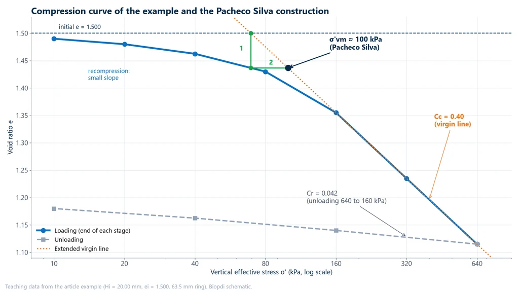
The practical reading is straightforward: if the structure's load takes the soil beyond the knee, settlement is calculated with Cc and is large; if it stays below it, Cr is used and settlement is small. In the example, Cc is almost ten times Cr, so each log cycle of stress in the virgin segment costs ten times more settlement than in the recompression segment.
How is the preconsolidation stress determined?
The preconsolidation stress σ'vm, also called preconsolidation pressure (σ'p in the English-language literature), is the highest vertical effective stress the soil has carried in its history, whether from a layer later removed by erosion, from groundwater level changes or from desiccation. It is not read directly: it is estimated by a graphical construction on the compression curve, and NBR 16853 provides two.
In the Casagrande method (1936), the point of minimum radius of curvature on the curve is chosen, and a horizontal line and the tangent to the curve are drawn through it. The bisector of the angle between them intersects the extension of the virgin compression line, and the abscissa of that intersection is σ'vm. The weakness of the method is precisely locating the point of minimum radius, which depends on the plot scale and on the eye of whoever draws it.
The Pacheco Silva method (1970), proposed in Brazil and widely used there, does without that point. It takes three lines, numbered in the chart above:
- draw a horizontal line at the initial void ratio ei and extend the virgin compression line until it intersects it;
- from that intersection, drop a vertical line down to the curve;
- from that point on the curve, draw a horizontal line to the extension of the virgin compression line. The abscissa of this last point is σ'vm.
When the virgin segment is strongly curved, NBR 16853 (note to 7.6.2) recommends applying the Pacheco Silva construction to the log(1 + e) versus log σ plot, as proposed by Martins (1983).
Whatever the method, σ'vm is an estimate. Umar and Sadrekarimi (2017, Canadian Geotechnical Journal) compared 11 graphical methods on 30 tests with preconsolidation imposed in the laboratory and concluded that most of them overestimate the true value. In practice, the method used is reported and the result is treated as a range, not an exact number.
What does the overconsolidation ratio indicate?
The overconsolidation ratio compares σ'vm with the current effective stress at the depth the sample came from: OCR = σ'vm/σ'v0. With OCR = 1, the clay is normally consolidated: any new load already falls on the virgin compression line. With OCR greater than 1, it is overconsolidated, and the structure has a stress "margin" within which settlement is small. Soft lowland clays typically have OCR close to 1 to 2 at depth and much higher values in the desiccated surface crust. If the test gives OCR less than 1, there are two explanations: the sample was disturbed, which flattens the curve and shifts the knee to the left, or the layer is still consolidating under a recent load.
How do you know whether the sample was good?
Sample quality is measured on the compression curve itself. The criterion of Lunne, Berre and Strandvik (1997) compares the initial void ratio e0 with the void ratio ev0 the specimen reaches when reloaded to the in situ effective stress σ'v0: the more the soil compresses just to return to its in situ state, the more its structure was disturbed during sampling, transport or trimming. The indicator is Δe/e0 = (e0 − ev0)/e0, and for clays with OCR from 1 to 2 the classification is:
| Δe/e0 (OCR from 1 to 2) | Sample quality |
|---|---|
| below 0.04 | very good to excellent |
| 0.04 to 0.07 | good to fair |
| 0.07 to 0.14 | poor |
| above 0.14 | very poor |
With the data from the worked example further on: e0 = 1.500 and σ'v0 = 55.3 kPa. Interpolating on a log scale between 40 and 80 kPa, the fraction is log(55.3/40)/log 2 = 0.467, and ev0 = 1.4625 − 0.467 × 0.0325 = 1.447. So Δe/e0 = (1.500 − 1.447)/1.500 = 0.053/1.500 ≈ 0.035: a very good to excellent sample, and the curve can be used without reservation. A disturbed sample would give a much larger Δe/e0, a rounded curve and an underestimated σ'vm, as described under common mistakes.
How are t50 and t90 read from the time curves?
For each load increment used for cv, the height readings are plotted as two curves. The two charts below show the same increment from the example, from 160 to 320 kPa: on the left, height versus the logarithm of time, with the Casagrande construction; on the right, height versus the square root of time, with the Taylor construction.
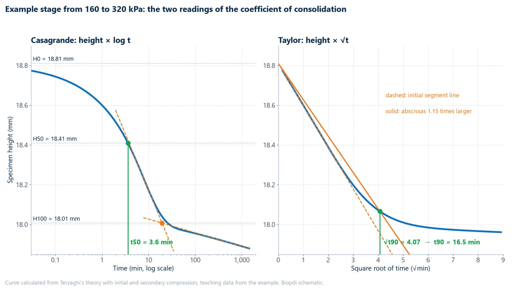
In the Casagrande construction, the end of primary consolidation, H100, is the intersection of the tangent to the steepest part of the curve with the tangent to the final secondary compression segment. The theoretical start, H0, comes from the parabolic shape of the beginning of the curve: two times t1 and t2 = 4·t1 are chosen, and H0 = H1 + (H1 − H2). NBR 16853 (7.4.2.3) only accepts this construction when the height change up to t2 is greater than one quarter and less than one half of the change over the increment. The mid height H50 = (H0 + H100)/2 marks t50 on the curve.
In the Taylor construction, the beginning of the √t curve is a straight line. That line is drawn, along with a second line from the same starting point with abscissas 1.15 times larger; where the second line crosses the curve is √t90. The drainage distance uses H50 = H0 − (5/9)·(H0 − H90), an expression given in NBR 16853 itself (7.4.3.4). Taylor is usually quicker to apply, because t90 appears before the increment ends; Casagrande requires waiting for the secondary segment, but it also provides Cα.
Which cv should be used in design?
The two methods give the same order of magnitude but rarely the same number, and neither one is "the right one". The cv also changes with stress level: in the overconsolidated range it is much higher than in the virgin range, and it differs between loading and unloading, as ASTM D2435 itself notes. That is why NBR 16853 requires the cv versus log average pressure curve, and design should use the value from the stress range the structure will impose. Even so, the field cv usually differs from the laboratory value, because the real layer has sand lenses, horizontal drainage and a scale the sample cannot reproduce. On major projects, the value is recalibrated using the embankment instrumentation.
How significant is secondary compression?
After primary consolidation ends, the soil keeps compressing under constant effective stress. On the height versus log time plot, this segment is a straight line, and its slope expressed in void ratio is the secondary compression index Cα = Δe/Δlog t. NBR 16853 requires readings to be extended until this line is defined when needed (6.5.5), but it does not calculate Cα; its value and use come from the literature. The secondary settlement of a layer between times t1 and t2 is:
ρs = H · Cα / (1 + ep) · log(t2/t1)
where ep is the void ratio at the end of primary consolidation and t1 is usually the time of the end of primary consolidation in the field. Mesri and Godlewski (1977) showed that the ratio Cα/Cc is practically constant for each soil, and Terzaghi, Peck and Mesri (1996) give Cα/Cc = 0.04 ± 0.01 for inorganic clays and silts, which allows Cα to be estimated when the test did not measure it.
With the data from the worked example further on: Cc = 0.40 gives Cα ≈ 0.04 × 0.40 = 0.016. At the end of primary consolidation in the field, the clay is at 135.3 kPa, and the virgin compression line gives ep = 1.355 − 0.3986 × log(135.3/160) ≈ 1.384. From t90 = 3.3 years to 30 years: ρs = 6 × 0.016/2.384 × log(30/3.3) = 0.0403 × 0.959 ≈ 0.039 m, about 4 cm, added to the 15 cm of primary settlement. In an inorganic clay of medium compressibility this contribution is small; in highly compressible clays, with Cc above 1, it reaches the order of 10 cm over the same interval, which is why structures on these deposits keep settling after the time calculated with Terzaghi's theory.
Worked example: from the readings to the settlement of the layer
The data below are for teaching only. We created them for this article and checked them by hand. They follow a complete test and end with the settlement of a clay layer under an embankment. The specimen sits in a 63.5 mm diameter ring, with initial height Hi = 20.00 mm and initial void ratio ei = 1.500. The diameter-to-height ratio is 3.2, which is within NBR 16853 (the Brazilian standard for the oedometer consolidation test) and DNER-IE 005/94 (the Brazilian highway department method).
1. Void ratio and compression indices
The height of solids is Hs = 20.00 / (1 + 1.500) = 8.000 mm. Each end-of-stage height becomes a void ratio through e = H/8.000 − 1. The table gives the readings and the results:
| Stage | Pressure (kPa) | Final height (mm) | Void ratio e |
|---|---|---|---|
| Loading | 10 | 19.92 | 1.490 |
| Loading | 20 | 19.84 | 1.480 |
| Loading | 40 | 19.70 | 1.4625 |
| Loading | 80 | 19.44 | 1.430 |
| Loading | 160 | 18.84 | 1.355 |
| Loading | 320 | 17.88 | 1.235 |
| Loading | 640 | 16.92 | 1.115 |
| Unloading | 160 | 17.12 | 1.140 |
| Unloading | 40 | 17.30 | 1.1625 |
| Unloading | 10 | 17.44 | 1.180 |
On the virgin compression line, between 160 and 320 kPa: Cc = (1.355 − 1.235) / log(320/160) = 0.120 / 0.301 = 0.40. Between 320 and 640 kPa the change is also 0.120, which confirms a straight virgin line. On unloading from 640 to 160 kPa: Cr = (1.140 − 1.115) / log 4 = 0.025 / 0.602 = 0.042, about one tenth of Cc.
2. Preconsolidation stress by Pacheco Silva and OCR
The virgin line is e = 1.355 − 0.3986·log(σ'/160). Following the three lines of the construction:
- horizontal at ei = 1.500: log(σ'/160) = −0.145/0.3986 = −0.364, so σ' = 69.2 kPa;
- vertical at 69.2 kPa up to the curve, interpolating in log between 40 and 80 kPa: the fraction is log(69.2/40)/log 2 = 0.791, and e = 1.4625 − 0.791 × 0.0325 = 1.437;
- horizontal at e = 1.437 to the virgin line: log(σ'/160) = (1.355 − 1.437)/0.3986 = −0.205, so σ'vm ≈ 100 kPa.
If the sample came from a point with σ'v0 = 55.3 kPa (calculated in step 5), OCR = 100/55.3 = 1.8: the clay is lightly overconsolidated.
3. Coefficient of consolidation in the 160 to 320 kPa stage
With the Casagrande construction on the log t plot, H0 = 18.81 mm and H100 = 18.01 mm, so H50 = 18.41 mm, read at t50 = 3.6 min = 216 s. The drainage path is Hd = 0.5 × 1.841 = 0.9205 cm, and Hd² = 0.847 cm². Then cv = 0.197 × 0.847 / 216 = 7.7 × 10⁻⁴ cm²/s.
With the Taylor construction, √t90 = 4.066 √min, so t90 = 16.5 min = 990 s, with H90 = 18.07 mm and H50 = 18.81 − (5/9) × 0.74 = 18.40 mm. With Hd = 0.920 cm and Hd² = 0.8464 cm²: cv = 0.848 × 0.8464 / 990 = 7.25 × 10⁻⁴ cm²/s, or 7.25 × 10⁻⁸ m²/s × 31.54 × 10⁶ s/year ≈ 2.29 m²/year.
The two methods differ by about 6%, which is within what is expected. For the time calculation in the field, the example uses the Taylor value, the lower one and therefore the more conservative for the time estimate.
4. Volume change and permeability
In the same stage, av = 0.120/160 = 7.5 × 10⁻⁴ kPa⁻¹ and mv = 7.5 × 10⁻⁴ / (1 + 1.355) = 3.2 × 10⁻⁴ m²/kN, using the void ratio at the start of the stage. With the mean value for the stage, as DNER-IE 005/94 does (e = 1.295), the result would be 3.27 × 10⁻⁴ m²/kN, about 3% higher, and k and Eoed would change in the same proportion. The indirect permeability is k = 7.25 × 10⁻⁸ m²/s × 3.185 × 10⁻⁴ m²/kN × 9.81 kN/m³ = 2.3 × 10⁻¹⁰ m/s (2.3 × 10⁻⁸ cm/s), a typical value for clay. The oedometric modulus for the stage is Eoed = 1/(3.185 × 10⁻⁴) ≈ 3,140 kPa, about 3.1 MPa.
5. Settlement and time of a clay layer in the field
The profile has the water table at the surface, 4 m of sand with γsat = 19 kN/m³, 6 m of clay with γsat = 16 kN/m³ and the parameters above, and sand at the base, which ensures double drainage. On top of it, a wide 4 m embankment with γ = 20 kN/m³ is built, adding Δσ = 4 × 20 = 80 kPa at every depth (one-dimensional condition).
- Stress at mid-depth of the clay (7 m): σ'v0 = 4 × (19 − 9.81) + 3 × (16 − 9.81) = 36.8 + 18.6 = 55.3 kPa. With the embankment, σ'vf = 135.3 kPa, above σ'vm = 100 kPa.
- Primary settlement: ρ = 6/(1 + 1.50) × [0.042 × log(100/55.3) + 0.40 × log(135.3/100)] = 2.4 × [0.0108 + 0.0526] = 0.152 m, about 15 cm. Almost all of it comes from the portion above σ'vm.
- Time: with Hd = 3 m and cv = 2.29 m²/year, t90 = 0.848 × 9 / 2.29 = 3.3 years and t50 = 0.197 × 9 / 2.29 = 0.77 year, about 9 months. If the base of the clay were impermeable, drainage would be through the top only, Hd would become 6 m and t90 = 0.848 × 36/2.29 ≈ 13.3 years: doubling the drainage path quadruples the time. That is why vertical drains, which shorten the path of the water, shorten the wait so much.
- Settlement after 1 year: Tv = 2.29 × 1 / 9 = 0.254; U = √(4 × 0.254/π) = 56.9%; ρ = 0.569 × 15.2 = 8.6 cm.
The result comes with three caveats that apply to any real project. The 6 m layer should be divided into sublayers, each with its own initial stress, instead of a single point at mid-depth. The calculation does not include secondary compression, which continues after primary consolidation and, as estimated in the interpretation section, adds about 4 cm over 30 years. And the laboratory cv, applied to the whole layer, is the largest source of uncertainty in the time estimate.
6. Check by correlation
For preliminary design, the Terzaghi and Peck (1967) correlation, adapted from Skempton, estimates Cc ≈ 0.009 · (LL − 10) for normally consolidated clay of low sensitivity. With a liquid limit of 54%, Cc ≈ 0.009 × 44 = 0.40, the same value as the test. The match is specific to this example: structured Brazilian clays often depart from these correlations, which serve to check the order of magnitude, never to replace the test.
Values measured in Brazilian soft clay
Compressibility parameters vary widely between soft clay deposits, and with depth within the same deposit, and this scatter is why every project needs its own test. A well-documented case is the instrumented embankment at Sarapuí (Rio de Janeiro state, Brazil), where Pessoa et al. (2023, Brazilian Journal of Development) measured Cc from 0.72 to 1.49 and OCR from 8.9 in the crust to 1.26 at 10.5 m depth. Back-analysis of the settlements gave cv from 5.5 to 12 × 10⁻⁴ cm²/s, against 20 × 10⁻⁴ cm²/s estimated at the start of construction. That is the order of magnitude of the example in this article, and also a reminder of how far the design cv can be off.
Common mistakes and limits of the test
Most poor consolidation results do not come from the calculation but from the sample and from how the curves are read. The most frequent mistakes are:
- Citing a withdrawn standard: following NBR 12007, withdrawn in 2015, or giving the wrong date for NBR 16853. The current edition is the 2020 one, reaffirmed in 2025.
- Disturbed sample: disturbance during sampling, transport or trimming flattens the curve, lowers Cc, raises Cr and erases the break at σ'vm. In a deposit in the Baixada de Jacarepaguá (Rio de Janeiro), a 50% to 80% reduction in the Cc of one investigation campaign was attributed to sample quality. The Δe/e0 criterion, explained in the interpretation section, measures this disturbance before the result goes into the design.
- Treating σ'vm as an exact measurement: it is a graphical construction, and the methods tend to overestimate it.
- Calculating cv where the curve does not follow Terzaghi: if the time curve does not have the S shape, NBR 16853 does not allow the calculation. With Casagrande, check the condition on t1 and t2.
- Using a single cv for the whole stress range: in the overconsolidated range it is much higher than on the virgin line.
- Interpreting time in unsaturated soil: ASTM D2435 notes that the time interpretation is valid only for a fully saturated specimen. Compacted or residual soil calls for a test with inundation and an assessment of collapse or swelling.
- Ignoring secondary compression: at Sarapuí, after about 1,000 days, the measured settlement exceeded the one calculated with primary consolidation alone.
- Applying the load increment with impact or too slowly: a transfer longer than 2 seconds, or with a shock, distorts precisely the first readings, which define H0.
- Letting the temperature vary: with readings in hundredths of a millimeter over several days, the thermal expansion of the apparatus shows up in the curve.
- Calculating settlement with a single point at mid-depth of a thick or overconsolidated layer, instead of subdividing it.
Consolidation, compaction and the other soil tests
Consolidation and compaction are often confused, but they are opposite processes in time. Compaction reduces the air voids through mechanical energy applied in seconds, as in the Proctor test, which determines the optimum moisture content and the maximum dry density of a soil. Consolidation reduces the water voids through a load sustained over hours in the laboratory and years in the field. On site, "consolidation of concrete" is something else: vibrating fresh concrete to expel entrapped air, unrelated to this test.
The consolidation test measures deformation under load, not strength. To know whether the soil fails, other tests come in. The triaxial test measures shear strength with control of drainage and pore pressure, and the direct shear test does the same more simply, on an imposed failure plane. In pavement engineering, the CBR test evaluates the bearing capacity of the compacted subgrade, the resilient modulus the elastic response under repeated loading, and the Marshall test the asphalt mixture.
Biopdi consolidation press
Biopdi manufactures the consolidation press in two models, as part of its line of soil testing equipment. The manual model has a lever for slotted weights of several capacities, up to 500 kgf (4.9 kN), and a dial gauge for the specimen height. The automatic electric model is the same machine as the CBR and Marshall test press, the PCM-5k press, which performs the consolidation test with the 2 or 3 inch cell: it runs the test from the settings entered on the touchscreen, holds the load constant in each stage, measures load with a load cell and height with an LVDT, and stores the tests on an SD card:
The automatic press in the consolidation test
Electromechanical, with a ball screw that applies the load and two threaded screws that position the crosshead, 300 mm test space width between columns, 50 kN (11,240 lbf) capacity, constant load control, 100 mm stroke and speed from 0.001 to 50 mm/min. Each part has a role in the test:

- Load cell measures the applied load; interchangeable from 5 to 5,000 kgf (0.05 to 49 kN)
- LVDT with 50 mm range and 0.01 mm resolution measures the height; the actuator encoder reads 0.001 mm
- Consolidation cell of 2 or 3 inches confines and drains the specimen
- Touchscreen sets maximum force, time and displacement; reads from 1/8 min to 24 h
- SD card and USB data to the computer and reports
- Limit switches and emergency stop upper and lower limits and stop button
Accessories for the consolidation test
The accessories below come with the consolidation presses, depending on the model:
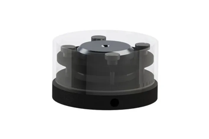
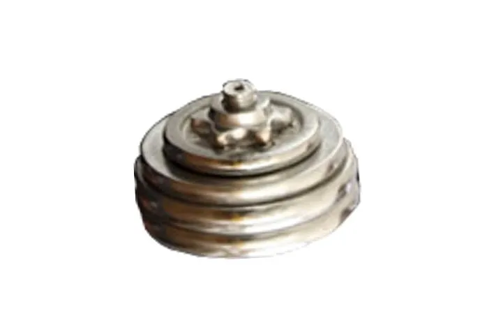
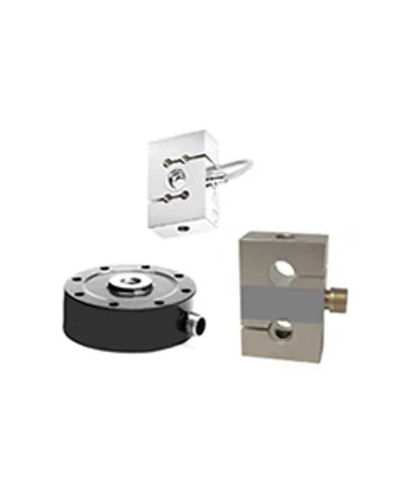
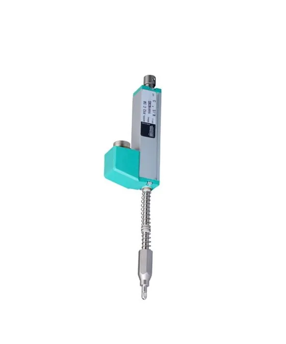
The 50 kN capacity of the frame is more than enough for the test, which, as the force table shows, rarely exceeds 10 kN. What needs sizing is the load cell. In a 63.5 mm ring taken to 1,280 kPa, the maximum force is 4.05 kN, and a 500 kgf (4.9 kN) load cell covers the test with better resolution in the low stages; in a 100 mm ring to the same pressure, the force reaches 10.05 kN and calls for the 2,000 kgf (19.6 kN) load cell. The configuration for each laboratory is defined in the quote, and our technical team answers questions through the contact page. For the other soil tests, Biopdi also manufactures the triaxial testing system, the direct shear apparatus and the CBR and Marshall test press.
Other tests and technical references
Resilient modulus (MR): what it is, how to calculate it and the repeated load test per Brazilian standards DNIT 134 and 135/2018
Resilient modulus (MR) is repeated deviator stress divided by recoverable strain in soils, aggregates and asphalt: MR = σd/εr, in MPa (DNIT 134, 135).
Marshall test: stability, flow, Vv, VMA (VAM) and VFA (RBV) per DNIT 447/2024-ME
The Marshall test measures the stability and flow of asphalt mixtures at 60 °C per DNIT 447/2024-ME. Procedure, Vv, VMA, VFA and a worked example.
CBR test and the California Bearing Ratio
CBR test (California Bearing Ratio): NBR 9895:2025 and DNIT 172 standards, procedure, formula with 6.9 and 10.35 MPa, worked example and CBR by layer.
Direct shear test: ASTM D3080 standard, step-by-step procedure and how to calculate c' and φ'
The direct shear test measures soil shear strength and gives the cohesion c' and friction angle φ'. ASTM D3080-23, step by step, with a worked example.
Frequently asked questions
What does consolidation mean?
Consolidation is the reduction in volume of a saturated soil caused by water slowly draining out of the pores when the soil is loaded. In clays, the process can take months or years, and on site it shows up as settlement.
What is consolidation theory?
It is Terzaghi's one-dimensional consolidation theory, published in 1925. A load increment creates excess pore water pressure, which dissipates through vertical drainage. Settlement follows this dissipation according to the time factor Tv = cv·t/Hd². This theory is what lets us calculate cv in the laboratory and predict how long settlement will take in the field.
What is consolidation in civil construction?
It is the slow settlement of embankments, buildings and pavements that rest on soft clay. The consolidation test predicts how much the structure will settle and how long it will take. Those two numbers determine whether a temporary surcharge or vertical drains are needed, and how long to wait before paving or building.
Are the consolidation test and the oedometer test the same thing?
Yes. "Oedometer" refers to the cell with a rigid ring that prevents lateral deformation of the sample while allowing drainage through its top and bottom faces. In NBR 16853 (the Brazilian standard for this test), the technical name is one-dimensional consolidation test.
Which standard covers the consolidation test?
In Brazil, it is ABNT NBR 16853:2020, Soil: one-dimensional consolidation test, reaffirmed in 2025. It replaced NBR 12007, which was withdrawn in 2015. DNIT (Brazil's National Department of Transport Infrastructure) has DNER-IE 005/94. Outside Brazil, the references are ASTM D2435/D2435M-25 for the incremental loading test and ASTM D4186/D4186M-20e2 for the controlled-strain test.
Is NBR 12007 still valid?
No. NBR 12007 was withdrawn on July 20, 2015, and its technical content was incorporated into ABNT NBR 16853:2020, which is the current reference for the consolidation test in Brazil.
What does NBR 5739 cover?
It is the Brazilian standard for compression testing of cylindrical concrete specimens, in its 2018 edition, reaffirmed in 2023. It does not apply to soil; the test is explained in the article on NBR 5739.
Which standard covers soil permeability testing?
In Brazil, ABNT NBR 14545 covers the permeability of clayey soils using the falling-head method, and ABNT NBR 13292 covers the permeability of granular soils using the constant-head method. In clay, permeability can also be measured directly in a fixed-ring consolidation cell, or estimated from the cv and mv obtained in the test.
How long does a consolidation test take?
Each load stage typically lasts 24 hours, with readings from 1/8 minute to 24 hours. A loading sequence from 10 to 640 kPa with three unloading stages adds up to about ten days, which is why the test takes one to two weeks in clays.
Which parameters does the consolidation test provide?
The compression index Cc, the recompression index Cr, the preconsolidation stress σ'vm (and, combined with the in-situ stress, the OCR), the coefficient of consolidation cv, the coefficient of volume compressibility mv, the oedometer (constrained) modulus Eoed = 1/mv and, indirectly, the permeability k = cv·mv·γw. The first parameters tell you how much the soil settles; cv tells you how long it takes.
Does the consolidation test calculate settlement?
Not directly. It provides Cc, Cr, σ'vm and cv, and the designer combines them with the layer thickness, the drainage conditions and the in-situ stresses before and after construction to calculate how much the structure settles and how long it takes, as in the worked example in this article.
How is the preconsolidation stress determined?
By graphical construction on the void ratio versus log stress curve, using the Casagrande (1936) or the Pacheco Silva (1970) method, both included in NBR 16853. The Pacheco Silva method uses a horizontal line at the initial void ratio and the extension of the virgin compression line, does not depend on locating the point of maximum curvature, and is widely used in Brazil; the Casagrande method is the most widely used internationally.
What is the difference between the Taylor and Casagrande methods for cv?
Casagrande uses the height versus log time curve and t50, with cv = 0.197·Hd²/t50. Taylor uses the height versus square root of time curve and t90, with cv = 0.848·Hd²/t90. Both give the same order of magnitude; Taylor's method gives a result sooner, while Casagrande's also provides secondary compression.
What are the types of consolidation test?
The incremental loading test, with the load doubled at each stage, covered by NBR 16853 and ASTM D2435 (methods A and B), and the continuous controlled-strain test, the CRS test of ASTM D4186, which measures pore pressure at the base and calculates cv and k throughout loading, but does not provide secondary compression. There are also variants with inundation to measure collapse and swelling.
What is the difference between consolidation and compaction?
Compaction reduces air voids through mechanical energy applied quickly, as in the Proctor test, and is done deliberately during construction. Consolidation reduces water-filled voids under a load sustained over time, and it happens on its own under the weight of the embankment or the structure.
Is the consolidation test valid for unsaturated soils?
The interpretation of time readings, and therefore cv, is only valid for a saturated specimen. In compacted or residual soils, the test is performed with inundation at a pressure that simulates field conditions, after the end of primary consolidation for that stage, as specified in NBR 16853, and the measured change in height is used to assess collapse or swelling.