
The resilient modulus (MR), also called the modulus of resilience in pavement engineering (resilient modulus), is the ratio between the deviator stress applied repeatedly to a soil, a crushed stone or an asphalt mixture and the strain the material recovers in each cycle: MR = σd / εr, in MPa, measured with load pulses of 0.1 s every second (1 Hz). It measures the elastic stiffness of the material under traffic and is the main stiffness input for mechanistic-empirical pavement design (MeDiNa, the Brazilian design method). Soils and crushed stone are tested in the repeated-load triaxial test according to DNIT 134/2018-ME (the Brazilian highway department standard for resilient modulus of soils); asphalt mixtures are tested in diametral compression according to DNIT 135/2018-ME (the Brazilian standard for resilient modulus of asphalt mixtures). As an order of magnitude, a fine-grained subgrade soil falls between 25 and 200 MPa, and an asphalt concrete between 2,000 and 12,000 MPa.
The name is misleading, because materials science uses the same expression for a different quantity. In metals, the modulus of resilience is the elastic energy the material stores per unit volume up to yielding, Ur = σe² / (2E), in J/m³, the subject of the article on resilience of materials. In pavement engineering, the resilient modulus is a stiffness, a stress divided by a strain, and this article deals with that second meaning.
In short:
- Formula: MR = σd / εr, with σd = P / A and εr = δr / H0.
- Loading: 0.1 s pulses followed by 0.9 s of rest, that is, 1 Hz, in both MR standards.
- Soils and crushed stone: 3 conditioning stress pairs with 500 cycles each and 18 stress pairs for the calculation (DNIT 134/2018-ME).
- Asphalt mixtures: diametral compression at 25 ± 0.5 °C, with a load between 5 % and 25 % of the tensile strength (DNIT 135/2018-ME).
- Permanent deformation: a separate test, with at least 150,000 cycles per specimen (DNIT 179/2018-IE, the Brazilian procedure for permanent deformation of soils).
The two meanings of "modulus of resilience"
The modulus of resilience of metals and the resilient modulus of pavement engineering share only the idea of elastic recovery. The one for metals is an area under the stress-strain curve of the tensile test, taken up to yielding; the one for pavements is a slope, measured at very small strains and under cyclic loading, nowhere near failure. That is why the units do not convert into each other: J/m³ has the same dimension as the pascal, but a value of 0.31 MJ/m³ for a steel and an MR of 150 MPa for a soil do not describe the same thing. The table compares the two quantities and adds the two that MR is most often confused with, CBR and the modulus of elasticity:
| Item | Metals (Ur) | Pavement engineering (MR) | CBR | Modulus of elasticity (E) |
|---|---|---|---|---|
| What it measures | elastic energy stored up to yielding | stiffness under repeated loading | resistance to penetration, compared with that of a standard crushed stone | stiffness under static loading, in the linear region |
| Formula | Ur = σe² / (2E) | MR = σd / εr | piston pressure / standard pressure × 100 | E = σ / ε |
| Usual unit | MJ/m³ or kJ/m³ | MPa | % | MPa or GPa |
| Where it comes from | tensile test (E and yield) | repeated-load triaxial test or diametral compression | piston penetration at constant speed (DNIT 172/2016-ME) | static tensile or compression test |
| Use | material selection for springs | mechanistic-empirical pavement design | empirical design and material screening | structural design of parts |
The confusion shows up even in glossaries that rank well in search results, which describe the MR of pavements as "absorbed energy". If the text talks about J/m³, springs or yield strength, it is the metals meaning; if it talks about deviator stress, confining stress, DNIT or subgrade, it is the meaning of this article.
Why pavements are tested under repeated loading
Pavements are tested under repeated loading because that is how traffic loads them: each wheel pass applies to a point of the pavement a load that rises and falls within fractions of a second. The layers deform and, once the wheel has passed, recover almost all of the deformation. The recovered part is the resilient deformation, elastic in nature (see elastic deformation); the small part that does not recover is the permanent deformation, which adds up with every pass and shows up on the surface as wheel-path rutting. DNIT 134/2018-ME defines resilient behavior precisely this way: the elastic response of the material to a load applied in short-duration pulses.
The two parts cause different distresses. The resilient part governs pavement deflection and the tensile strain at the bottom of the asphalt surface layer, which, repeated millions of times, leads to fatigue and cracking. The permanent part governs rutting. A rational design method therefore needs the stiffness of each layer measured under traffic conditions: short, repeated loading, with small strains and under the confinement the layer has in the pavement. That is what the resilient modulus provides.
The CBR test (California Bearing Ratio, known in Brazil as Índice de Suporte Califórnia, ISC), the basis of the 1981 empirical method of the former DNER (Brazil's former National Highway Department), does something else: it drives a piston into the soil at constant speed, with displacements of millimeters, and measures a resistance to penetration. Two soils with the same CBR can have very different stiffness under repeated loading. The test is detailed in the article on the CBR test; here the conclusion of the MeDiNa testing guide (DNIT, 2026) is enough: it does not recommend correlations between MR and CBR because of the poor consistency between the two parameters.
The repeated-load triaxial test was developed by Seed and co-workers in the United States starting in the 1950s. The name "resilient modulus" was adopted to distinguish this quantity from the Young's modulus obtained under static loading, and in Brazil the test has been performed since 1977 at COPPE/UFRJ, according to Bernucci and co-workers (Pavimentação Asfáltica: formação básica para engenheiros, ch. 7).
Resilient modulus formula and how to calculate it
The calculation of the resilient modulus uses two stresses from the triaxial test, the confining stress and the deviator stress, and one strain, the resilient strain. In the triaxial test, the cylindrical specimen sits inside a chamber with pressurized air. This pressure acts on all faces and is the confining stress, σ3, which represents the lateral confinement of the layer in the pavement. On top of it, a piston applies vertical pulses. The total vertical stress is σ1, and the difference σ1 − σ3 is the deviator stress, σd: it is the part of the vertical stress that exceeds the confinement, the part that actually tends to distort the material. DNIT 134/2018-ME defines MR as the ratio between the repeatedly applied deviator stress and the corresponding recoverable vertical strain:
MR = σd / εr
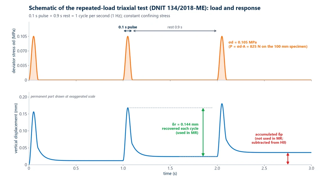
The deviator stress is the cyclic load divided by the cross-sectional area of the specimen, σd = P / A. The resilient strain is the displacement recovered in the cycle, δr, divided by the gauge reference height, H0: εr = δr / H0. The resilient displacement is measured by two LVDT displacement transducers attached to the specimen, between the point of maximum stress and the end of unloading. The reference height is the gauge length of the displacement transducer (the total height, if the transducer runs from top to bottom, or the middle-third length) minus the permanent displacement already accumulated. The table summarizes the quantities:
| Quantity | Expression | Unit |
|---|---|---|
| Resilient modulus | MR = σd / εr | MPa |
| Deviator stress | σd = σ1 − σ3 = P / A | MPa (N/mm²) |
| Resilient strain | εr = δr / H0 | dimensionless |
| Permanent strain | εp = δp / H0 | dimensionless or % |
The diagram below shows what the test records. At the top, the deviator stress pulses, each lasting 0.1 s followed by 0.9 s of rest. At the bottom, the vertical displacement: with each pulse the specimen shortens and, during the rest period, recovers the resilient part, δr, which is the one used in MR; the little that does not recover accumulates from cycle to cycle and has been drawn at an exaggerated scale so that it is visible.
For a linear elastic material, MR equals the modulus of elasticity, which is the remark made in the MeDiNa guide. Soils and crushed stone, however, are not linear: the MR of the same material changes with the confining stress and the deviator stress, which is why the test applies several stress pairs instead of just one. The relationship between stress and strain in general is covered in the article on the stress-strain curve.
Exercise 1: MR for one stress pair
Illustrative data. Soil specimen 100 mm in diameter and 200 mm high, LVDTs from top to bottom (H = 200 mm). Stress pair σ3 = 0.035 MPa and σd = 0.105 MPa. Up to this pair, the accumulated permanent displacement is 0.40 mm. Averaged over the cycles read, the resilient displacements are 0.140 mm on LVDT 1 and 0.148 mm on LVDT 2.
- Area: A = π × 50² = 7,853.98 mm². The cyclic load applied by the piston is P = 0.105 × 7,853.98 = 824.7 N.
- Resilient displacement: average of the two LVDTs, δr = (0.140 + 0.148) / 2 = 0.144 mm.
- Reference height: H0 = 200 − 0.40 = 199.60 mm.
- Resilient strain: εr = 0.144 / 199.60 = 7.214 × 10⁻⁴.
- MR = 0.105 / 7.214 × 10⁻⁴ = 145.5 MPa, about 146 MPa.
The value falls within the MeDiNa guide's range for fine-grained subgrade soils (25 to 200 MPa). Without subtracting the 0.40 mm, H0 = 200 mm and MR would come out at 145.8 MPa: the difference is small here, but it grows when the specimen accumulates several millimeters of permanent deformation.
Repeated load triaxial test on soils (DNIT 134/2018-ME)
The repeated load triaxial test, also called the dynamic triaxial test, determines the MR of soils and crushed stone by applying short pulses of deviator stress to a confined cylindrical test specimen without taking it to failure. The triaxial test in general, including the static types (UU, CU and CD) used for shear strength, is covered in the article on the triaxial test. The repeated load version uses the same idea of a membrane-encased specimen confined in a cell, but it replaces slow loading to failure with pulses. DNIT 134/2018-ME (approved on July 25, 2018, corrected version with Erratum 1 on April 20, 2023) is the Brazilian standard for the test. It replaced DNIT 134/2010-ME and is publicly available on the DNIT (Brazil's National Department of Transport Infrastructure) website.
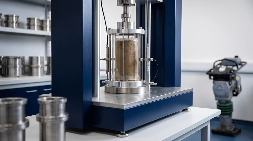
The photo shows a compacted soil specimen inside the triaxial cell, encased in a membrane. The cell pressure applies the confining stress, the piston at the top applies the load pulses, and the two LVDTs measure how much the specimen shortens and recovers with each pulse.
Materials and test specimen
The standard applies to soils, graded crushed stone, granular stabilized materials and soils improved with small chemical additions or fibers, provided they are not chemically stabilized. Soil-cement, cement-treated graded crushed stone and other cemented materials have their own standard, DNIT 181/2018-ME. In that standard the test is run without confining stress, as an unconfined compression test with repeated loading at 1 Hz, at five stress levels, after curing (typically 7 and 28 days for cement). The key points that define the test specimen are:
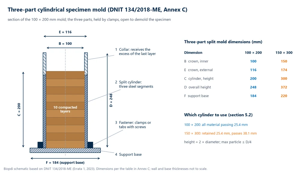
- Dimensions: a 100 × 200 mm cylinder for soil without gravel or material that fully passes the 25.4 mm sieve; a 150 × 300 mm cylinder when there is material retained on 25.4 mm and everything passes 38.1 mm. In both cases the height is twice the diameter, and the maximum particle size does not exceed 1/4 of the diameter. If up to 10% of the material is retained on the 38.1 mm sieve, that fraction is discarded and the 150 mm cylinder is used; if up to 10% is retained on 25.4 mm and there is not enough material for the large cylinder, the retained fraction is discarded and the specimen is tested in the 100 mm cylinder, with this recorded in the report (DNIT 134, item 5.2).
- Molding: compaction in a three-part steel split mold, in 10 layers, with a standard Proctor rammer (2,500 g, 305 mm drop) or modified Proctor rammer (4,536 g, 457 mm drop), using the number of blows that gives the specified energy.
- Moisture content: the homogenized soil rests for at least 12 h in a moist room before compaction (not required for crushed stone). The moisture content measured on the specimen after the test may differ from the optimum by up to ± 1% for granular material and ± 0.5% for fine material. For gravelly soil and crushed stone, DNIT 134 requires the compaction curve to be obtained in a cylinder of the same size as the test specimen; the procedure in the split mold is given in DNIT 443/2023-ME. A curve obtained in the traditional Proctor cylinder, which has different dimensions, may indicate a different optimum moisture content.
The diagram below shows the split mold in cross section, with the dimensions from the table in Annex C of DNIT 134 for both specimen sizes. Note the collar at the top, which holds the excess from the last of the 10 layers, and the three parts of the cylinder, held by clamps at the base, which open to demold the specimen.
Required equipment
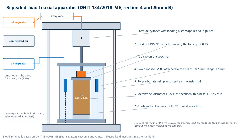
The standard describes a pneumatic press, with a compressed air cylinder and loading piston, and also accepts a hydraulic press capable of applying repeated loads. The pulse is generated by a three-way valve controlled by an electronic timer, and two pressure regulators set the deviator stress and the confining stress. The other requirements are:
- Triaxial cell made of polycarbonate or another material that allows the specimen to be seen, with metal base and top plate and a drainage port in the base.
- Load cell inside the cell, in direct contact with the top cap, with an accuracy of ± 0.5% of the measured value. The practical reason is that, inside the cell, the reading does not include the friction of the piston in the top plate seal.
- Two LVDTs (inductive displacement transducers, from the same family described in the article on the extensometer) in diametrically opposite positions, attached to the top cap and supported on guide rods or fixed in the middle third. The LVDT and acquisition system must read with a precision of 0.001 mm over a range of up to ± 5 mm, and the calculation uses the average of the two.
- Membrane of rubber or latex with an unstretched diameter of at least 95% of the specimen diameter and a thickness of at most 0.8% of it, plus a vacuum system to check whether it is punctured.
The following diagram brings these parts together in the setup from Annex B of the standard. Note the load cell inside the cell, resting on the top cap, the two LVDTs attached to the top cap and guided by rods down to the base, and the two air circuits: one regulator and the three-way valve form the σd pulse, and the other regulator keeps σ3 constant in the cell.
The test described is drained: the base valve stays open to the atmosphere throughout loading.
Conditioning and the 18 stress pairs
The whole test runs at 1 Hz, with a 0.1 s pulse and 0.9 s rest (60 cycles per minute), and the confining stress stays constant, without cycling. It has two phases:
- Conditioning: 500 repetitions of each of three (σ3; σd) pairs: 0.070 and 0.070 MPa; 0.070 and 0.210 MPa; 0.105 and 0.315 MPa. It eliminates the permanent deformations from the first load applications, which do not represent the material in service. For subgrade soils, the standard allows conditioning with only the first pair.
- MR determination: 18 stress pairs, six confining stress levels (0.020, 0.035, 0.050, 0.070, 0.105 and 0.140 MPa) and, for each one, deviator stresses that bring the σ1/σ3 ratio to 2, 3 and 4. The most severe pair has σ3 = 0.140 MPa and σd = 0.420 MPa. For subgrade, at the designer's discretion, the 12 pairs of the first four confining levels are sufficient.
The chart below plots the pairs in the σ3 × σd plane, numbered in the order in which the standard applies them. Each dashed line groups the pairs with the same σ1/σ3 ratio; the diamonds are the three conditioning pairs, which coincide with pairs 10, 12 and 15; and the blue band marks the 12 pairs that are sufficient for subgrade.
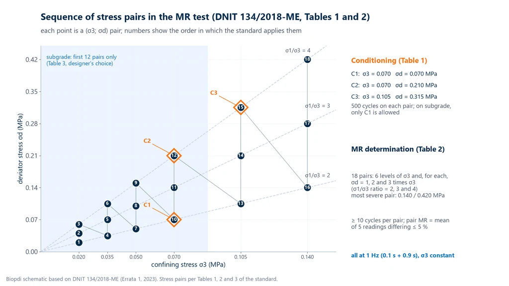
For each pair, at least 10 cycles are applied and at least 5 repetitions are recorded whose readings do not differ from each other by more than 5%; the MR of the pair is the average of these 5. If, at any phase, the accumulated permanent deformation reaches 5% of the specimen height (10 mm in the 200 mm cylinder, 15 mm in the 300 mm cylinder), the test is stopped and the result is discarded. At the end, the specimen goes into the oven at about 110 °C for 48 h, or until constant mass, to check the moisture content. When the sample is the only one from the borrow source or borehole, the standard recommends testing three identical specimens.
The result is not a single number: it is 18 MR values, one per pair, which the standard allows to be expressed by a mathematical relationship with the stresses, obtained by regression, and which design with MeDiNa (DNIT's mechanistic-empirical pavement design method) uses in that form. That is the subject of the next section.
Constitutive models: why MR depends on stresses
A resilient behavior model is the expression that gives the MR of a material as a function of the stresses acting on it, fitted by regression to the values measured in the test. A granular material, such as graded crushed stone, gains stiffness when confined: the grains are pressed more tightly against each other and the contacts between them stiffen. A fine clayey soil tends to lose stiffness as the deviator stress increases, because distortion grows faster than stress. Constitutive models capture these two effects with power expressions fitted to the 18 pairs. The MeDiNa guide (DNIT, 2026) uses the general model:
MR = k1 · σ3k2 · σdk3 · θk4
where θ = σ1 + 2σ3 is the first stress invariant (the sum of the three principal stresses), with stresses in MPa. Setting exponents to zero gives the particular cases:
- Constant MR (k2 = k3 = k4 = 0): linear elastic behavior, the simplest.
- Dependent on σ3 (k3 = k4 = 0): typical of granular materials.
- Dependent on σd (k2 = k4 = 0): typical of cohesive fine soils.
- Dependent on θ (k2 = k3 = 0): the "k-θ" model, a classic for crushed stone.
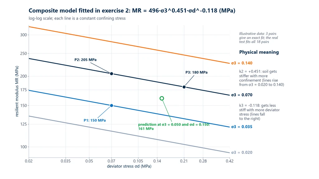
- Composite model (k4 = 0): MR = k1·σ3k2·σdk3, which covers both effects and is the most widely used in Brazil.
The sign of the exponents has a physical meaning: a positive k2 means the material stiffens with confinement; a negative k3, that it softens with deviator stress. In the United States, the AASHTO mechanistic-empirical guide uses the universal model from the NCHRP 1-37A project, MR = k1·pa·(θ/pa)k2·(τoct/pa + 1)k3, which normalizes stresses by atmospheric pressure pa and uses the octahedral shear stress τoct. The parameters of one model are not valid in the other. The literature also has other forms, such as that of Witczak and Uzan (1988), with the first invariant and the octahedral stress, and that of Witczak and Rada (1981); laboratory software often fits several of them to the same 18 pairs to compare R².
The fit is done by regression. Taking logarithms, the composite model becomes linear: ln MR = ln k1 + k2·ln σ3 + k3·ln σd, and a multiple linear regression on the 18 pairs gives the three parameters and the coefficient of determination R². Direct nonlinear regression is also used. The DNIT 134 report (Annex E) gives, for each pair, the recoverable displacement, the resilient strain and the MR, plus the LVDT reference height and the accumulated permanent displacement. When the results are expressed by a model, it is good practice to also report the parameters, the stress unit and R².
Exercise 2: fitting the composite model with three pairs
Illustrative data for a single soil: P1 (σ3 = 0.035; σd = 0.070 MPa) with MR = 150 MPa; P2 (0.070; 0.070) with 205 MPa; P3 (0.070; 0.210) with 180 MPa. Fit MR = k1·σ3k2·σdk3 and estimate the MR at σ3 = 0.050 and σd = 0.150 MPa.
- From P1 to P2 only σ3 changes, and it doubles: 205 / 150 = 2k2, so k2 = ln 1.3667 / ln 2 = 0.451.
- From P2 to P3 only σd changes, and it triples: 180 / 205 = 3k3, so k3 = ln 0.8780 / ln 3 = −0.118.
- With P2: k1 = 205 / (0.0700.451 × 0.070−0.118) = 205 / (0.3016 × 1.3700) ≈ 496 MPa.
- Check at P1: 496 × 0.0350.451 × 0.070−0.118 = 496 × 0.2207 × 1.3700 = 150.0 MPa.
- Prediction: 496 × 0.0500.451 × 0.150−0.118 = 496 × 0.2592 × 1.2518 ≈ 161 MPa.
With three points and three unknowns, the fit passes exactly through the points and says nothing about the quality of the model. In the real test, the 18 pairs give 15 degrees of freedom and R² becomes meaningful.
The chart below plots the fitted model on a log-log scale, where each confining stress becomes a straight line. The lines rise from σ3 = 0.020 to 0.140 MPa, which is the effect of a positive k2, and slope downward to the right, which is the effect of a negative k3. The open circle is the prediction from item 5, between the 0.035 and 0.070 MPa lines.
Asphalt mixtures: indirect tensile test (DNIT 135/2018-ME)
The resilient modulus of asphalt mixtures is measured by repeated-load indirect tension (diametral compression), because in the surface course the stress that governs fatigue is the tension at the bottom of the layer, which bends under the wheel. The indirect tensile test reproduces this tension in the laboratory: a cylindrical test specimen, laid on its side, is loaded along two opposite generatrices, and the vertical diametral plane is subjected to nearly uniform horizontal tension in its central region. It is the same principle as the indirect tensile strength test (splitting test, DNIT 136/2018-ME), only with small load pulses that do not break the specimen. DNIT 135/2018-ME (a test method of DNIT, Brazil's Department of Transport Infrastructure, approved on 04/26/2018 and replacing DNIT 135/2010-ME) defines the MR of the mixture as the ratio between the horizontal stress produced by the cyclic load and the corresponding recoverable horizontal strain.
Procedure
The test specimens are molded in the Marshall compactor (see the Marshall test) or in the gyratory compactor, or cored from the pavement. The procedure in the standard is as follows:
- Test specimen: diameter of 101.6 ± 3.8 mm and height between 35 and 70 mm, measured with a caliper (average of 4 readings). Stored for 24 h to 30 days at no more than 30 °C.
- Tensile strength: determine the indirect tensile strength (RT) per DNIT 136 on at least 3 identical specimens. The cyclic load of the MR test is set between 5% and 25% of this average RT.
- Temperature: at least 4 h in the chamber at the test temperature, usually 25 ± 0.5 °C. The chamber must hold 10 to 50 °C with an accuracy of 0.5 °C.
- Setup: specimen centered between concave steel loading strips 12.70 mm wide, with a fixed seating load of 25 to 75 N.
- Loading: haversine pulse of the form (1 − cos θ)/2, with 0.1 s of loading and 0.9 s of rest. First, 50 conditioning cycles; then, without interruption, 15 cycles, another 15 with the load 5% higher and another 15 with a further 5%, recording load and displacements at a rate of at least 200 points per second.
- Acceptance criterion: the MR is calculated over the last 5 cycles of each set of 15; the averages of the three sets may not differ by more than 5% from the overall average.
Displacement is measured with an LVDT with a minimum resolution of 0.0004 mm, either external (on a yoke clamped to the specimen) or internal (glued to both faces, with four sensors and a gauge length of 1/2 or 1/4 of the diameter; in this case the specimen is molded 10 mm taller and its faces are sawn). If the vertical displacement is also measured, Poisson's ratio is calculated; with only the horizontal sensor, 0.25 or 0.30 is assumed at 25 °C, and a note in the standard records that the Brazilian database uses 0.30. The load cell must have a minimum sensitivity of 0.5% of the maximum test load, and the result for the mixture is the average of at least 3 specimens.
MR, instantaneous modulus and total modulus
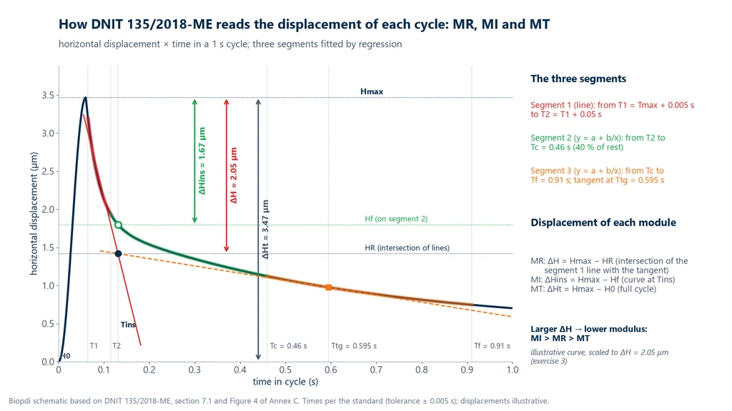
The horizontal displacement × time curve of each cycle does not return to zero all at once: it has a nearly linear unloading portion, a transition curve and a slow, viscous recovery during the rest period. The standard divides the curve into these three segments, fits a regression to each and defines three moduli with the same numerator and different displacements:
- Resilient modulus (MR): uses the displacement at the point where the unloading line crosses the tangent to the viscous recovery (taken at 0.595 s into the cycle). It is the design value, kept by Brazilian practice since the first standard of DNER (the former Brazilian highway department), in 1986.
- Instantaneous modulus (MI): uses the instantaneous displacement, read on the transition segment at that same instant.
- Total modulus (MT): uses the total displacement of the cycle, from the start of the pulse to the maximum, and therefore comes out lower.
The chart below performs this reading on an illustrative cycle. The line of segment 1 and the tangent to segment 3 at 0.595 s intersect at Tins: the height of this intersection gives the MR displacement, the curve at the same instant gives the MI displacement and the whole cycle gives the MT displacement. Since the MI displacement is the smallest and the MT displacement the largest, the moduli rank MI > MR > MT.
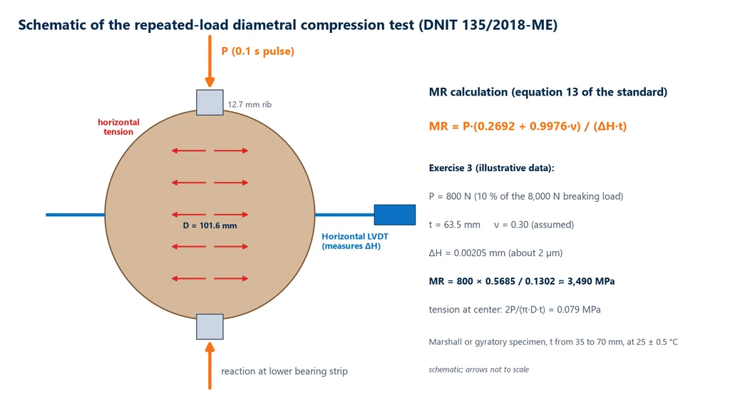
For the 101.6 mm specimen with an external LVDT, equation 13 of the standard gives the MR in MPa:
MR = P · (0.2692 + 0.9976·ν) / (ΔH · t)
where P is the cyclic load in N, ΔH the resilient horizontal displacement in mm, t the specimen height in mm and ν Poisson's ratio. The diagram below brings together the setup and the calculation: the vertical load P enters through the loading strips, produces horizontal tension along the vertical diameter, and the LVDT measures the change in the horizontal diameter, ΔH. Next to it are the equation and the numbers of the following exercise.
Exercise 3: MR of an asphalt mixture
Illustrative data. Marshall specimens with D = 101.6 mm and t = 63.5 mm. In the DNIT 136 test, three identical specimens failed at an average load F = 8,000 N. In the MR test, a cyclic load of 10% of the failure load is used, ν = 0.30 (no vertical sensor), and the external LVDT records ΔH = 0.00205 mm.
- RT = 2F / (π·D·t) = 16,000 / (π × 101.6 × 63.5) = 16,000 / 20,269 = 0.789 MPa.
- P = 0.10 × 8,000 = 800 N. The tension it produces at the center is 2 × 800 / 20,269 = 0.079 MPa, which is 10% of RT, within the 5% to 25% range.
- MR = 800 × (0.2692 + 0.9976 × 0.30) / (0.00205 × 63.5) = 800 × 0.5685 / 0.1302 = 3,494 MPa, about 3,490 MPa.
The measured displacement is about 2 µm. The minimum required resolution, 0.0004 mm, is one fifth of this signal, which is why sensor mounting, loading strip alignment and averaging over several cycles weigh so heavily on the result. The value falls within the range for asphalt concrete in the MeDiNa guide (Brazil's mechanistic-empirical pavement design method): 2,000 to 12,000 MPa.
How much does the assumed ν change this result? With only the horizontal sensor, DNIT 135 allows 0.25 or 0.30, and the choice goes straight into the factor of equation 13:
- With ν = 0.30: 0.2692 + 0.9976 × 0.30 = 0.5685, and MR = 3,494 MPa, as above.
- With ν = 0.25: 0.2692 + 0.9976 × 0.25 = 0.5186, and MR = 800 × 0.5186 / 0.1302 = 3,187 MPa, about 3,190 MPa.
- Ratio: 0.5685 / 0.5186 = 1.096. With the same load and displacement, the MR comes out about 9.6% higher with ν = 0.30.
The difference comes only from the assumption, not from the material. That is why the report must state whether ν was measured or assumed, and which value was used; two laboratories testing the same mixture with different assumed ν values will report MR results nearly 10% apart.
Permanent deformation (DNIT 179/2018-IE)
Permanent deformation is the portion of strain that is not recovered in each cycle and that, accumulated over millions of wheel passes, becomes rutting. It is measured in a separate test, on the same repeated-load triaxial equipment, per DNIT 179/2018-IE (a Brazilian test instruction approved on 05/15/2018, with Erratum 1 of 04/20/2023). Instead of many stress pairs with few cycles, a single stress pair is applied to each specimen for many cycles, recording the accumulated permanent strain, the subject of the article on plastic deformation. The main points of the standard are:
- Frequency: 2 Hz recommended (0.1 s pulse and 0.4 s rest), with 1 to 5 Hz allowed, the pulse always lasting 0.1 s and only the rest period adjusted, provided all tests on the same sample use the same frequency.
- Initial procedure: 50 cycles with σ3 = σd = 30 kPa, to seat the piston and top cap. The deformation in this phase is not counted, and the reference height is corrected.
- Test: at least 150,000 cycles per specimen, with intermediate readings (1, 2, 3... 100, 200... 1,000, 2,000... cycles) to describe the curve.
- Stress pairs: σ3 of 40, 80 and 120 kPa, each with a σ1/σ3 ratio of 2, 3 and 4, that is, σd equal to 1, 2 and 3 times σ3, up to 360 kPa. That makes 9 specimens, one per pair, with a minimum of 6 if the stresses are well spaced.
The results feed the Guimarães (2009) model, εp(%) = ψ1·(σ3/ρ0)ψ2·(σd/ρ0)ψ3·Nψ4, where ρ0 is the reference atmospheric pressure and N the number of cycles, fitted by multiple nonlinear regression. The standard also classifies the response into four types: I, shakedown (shakedown) after few cycles; II, shakedown after accumulating a large displacement; III, continuous accumulation, without stabilizing; IV, incremental collapse after few cycles. Shakedown is checked on the plot of the permanent strain rate versus the accumulated strain. The sum of the permanent deformations of each layer, multiplied by their thicknesses, gives the predicted rut depth.
Exercise 4: machine time
How much equipment time does the characterization of a material under the two soil standards take?
- Permanent deformation at 2 Hz: 150,000 / 2 = 75,000 s, or 20.8 h per specimen. With 9 specimens, 187.5 h, about 7.8 days of continuous operation.
- If the whole sample is tested at 5 Hz, the maximum allowed: 150,000 / 5 = 30,000 s, 8.3 h per specimen and 75 h for all 9. At 1 Hz, it would be 41.7 h per specimen.
- Resilient modulus at 1 Hz: 3 × 500 conditioning cycles plus at least 18 × 10 cycles = 1,680 cycles, or about 28 min of loading per specimen.
For anyone planning the laboratory, permanent deformation is the bottleneck: the MR of a material is done in one shift, while permanent deformation ties up the press for more than a week.
Typical values and use in pavement design (MeDiNa)
MeDiNa (Método de Dimensionamento Nacional, Brazil's national pavement design method) is the mechanistic-empirical design program of DNIT (Brazil's National Department of Transport Infrastructure). It calculates the stresses and strains in each layer with multilayer elastic theory (the AEMC routine) and compares these responses with fatigue damage and permanent deformation models. It came out of a cooperation agreement between IPR and COPPE/UFRJ (2015 to 2018). DNIT released version 2.0, recalibrated with UnB, on October 24, 2025, with the overlay design mode temporarily removed. The DNIT and UnB testing guide (2026) records that the method was implemented in 2025.
On DNIT new-construction projects, the use of MeDiNa is governed by service instruction IS-247 (Studies for the preparation of new-construction projects using the National Design Method). This is a specific instruction that supplements those in Publication IPR-726. It lists MR among the mandatory tests for the subgrade, borrow pits, graded crushed stone and asphalt mixtures, and it states plainly that the MeDiNa database, or data from academic work, does not replace testing. In practice, the MR of each layer becomes a design input, not a test that supplements the CBR. The parameters for each layer come from these standards:
| Layer | Stiffness parameters | Other parameters |
|---|---|---|
| Granular layers and subgrade | ν and k1 to k4 (DNIT 134), or constant MR | ψ1 to ψ4 (DNIT 179) |
| Chemically stabilized layers | ν and MR (DNIT 181) | ITS (DNIT 136) and fatigue (DNIT 434) |
| Asphalt mixtures | ν and MR (DNIT 135) | ITS (DNIT 136) and fatigue (DNIT 183) |
When a layer is described by a nonlinear model, the program starts from an initial MR, calculates the stresses, recalculates MR with the model and repeats until it converges. The MR adopted is the one at the center of the layer. MR can also be obtained in the field: deflection basins measured with a Benkelman beam or a falling weight deflectometer (FWD) are fed into the backcalculation program (BackMeDiNa). The guide rates a fit as good when the RMS error is below 5%, fair from 5% to 10% and unsatisfactory at 10% or more. There are also field stiffness gauges, such as the GeoGauge, which give a single, quick modulus that is useful for construction quality control. On a trial section with a fly ash and lime base in Ceará, Brazil, the correlation between this field modulus and the laboratory MR reached R² = 0.90, but the authors themselves did not recommend the equation because the dataset was small (Fernandes and co-authors, ANPET Congress, 2019). The field gauge gives a constant value; the laboratory MR is a function of stress, and that function is what MeDiNa uses.
For preliminary design, or to check whether a laboratory result is plausible, the MeDiNa guide gives modulus ranges by material (table 12, adapted from PMSP 2004, DER-SP 2006 and Bernucci et al. 2022). They do not replace testing the project's own material:
| Material | Modulus range (MPa) |
|---|---|
| Asphalt concrete | 2,000 to 12,000 |
| Cement-treated graded crushed stone | 5,000 to 15,000 |
| Granular materials | 100 to 500 |
| Fine-grained soils in base and subbase | 150 to 300 |
| Fine-grained soils in subgrade and subgrade reinforcement | 25 to 200 |
In table 2, the same guide lists ranges and typical values of Poisson's ratio by material, adapted from Huang (2004). Since pavement response is not very sensitive to variations in ν, the typical values in the table below are usually adopted in design:
| Material | Range of ν | Typical value |
|---|---|---|
| Asphalt concrete | 0.30 to 0.40 | 0.30 |
| Granular materials | 0.30 to 0.40 | 0.35 |
| Cement-treated granular materials | 0.10 to 0.20 | 0.15 |
| Cement-treated fine-grained soils | 0.15 to 0.35 | 0.25 |
| Lime-stabilized materials | 0.10 to 0.25 | 0.20 |
| Loose or silty sand | 0.20 to 0.40 | 0.30 |
| Dense sand | 0.30 to 0.45 | 0.35 |
| Fine-grained soils | 0.30 to 0.50 | 0.40 |
What IS-247 requires from the laboratory
IS-247 sets how many samples of each material go through each test. The table brings together the requirements related to MR and permanent deformation at the basic design stage. The instruction counts samples, not specimens: each test follows its own standard, and DNIT 179, for example, uses up to 9 specimens per material.
| Material | Resilient modulus | Permanent deformation and others |
|---|---|---|
| Subgrade | all samples from the boreholes (DNIT 134) | DNIT 179 on 10% of the samples tested for MR, at least 3 |
| Borrow pits and soil blends for base and subbase | 9 samples, from different boreholes in the borrow pit (DNIT 134) | 3 samples (DNIT 179) |
| Graded crushed stone for base | 3 samples (DNIT 134) | 1 sample (DNIT 179) |
| Materials stabilized with chemical additives | 3 samples (DNIT 181) | fatigue; unconfined compression at 7 days and splitting tensile test, 3 samples each |
| Asphalt mixtures | 1 test with 3 samples (DNIT 135) | flow number, 3 samples (DNIT 184); fatigue, 12 samples at 4 stress levels (DNIT 183) |
Two criteria in the same instruction change the laboratory's routine. In the subgrade, homogeneous segments are defined by a coefficient of variation of no more than 20% of the mean of the 18 stress pairs in each MR test, which requires the full test at every point. And MR may be waived for embankment material located more than 2.0 m below the subgrade leveling layer. Asphalt mixture specimens may be compacted in a Marshall compactor or a gyratory compactor, except for flow number specimens, which must come from the gyratory compactor only.
How to interpret the resilient modulus
Interpreting a resilient modulus requires knowing the stresses, moisture content, density and temperature at which it was measured, because the same material gives different values under each condition. The questions below are the ones that come up most often when reading reports and when moving from the laboratory to design.
Is MR the modulus of elasticity of the soil?
Only in the particular case of a linear elastic material. The modulus of elasticity of a steel is practically a material constant; the MR of a soil depends on the stress state and on the moisture content and density at which the specimen was compacted. That is why MR always comes with the stresses or the model, and a "soil MR" without this information cannot be used in design.
Why does the same soil have several MR values?
Because each stress pair gives one value, and in the pavement each depth has a different confining pressure and deviator stress. The 18 values from the test are points on a surface that the model describes; the value used in the calculation is the one the program finds for the stress state at the center of the layer.
Is a higher MR always better?
Not necessarily. In the subgrade and the granular layers, higher stiffness reduces deflections. In the surface course, a stiffer mixture takes a larger share of the wheel stress and may work under higher tension; if the fatigue resistance of that mixture does not keep up, service life drops. That is why MeDiNa evaluates MR together with the mixture's fatigue curve and the stiffness of the layers below, not in isolation.
Does the laboratory MR apply in the field?
It applies to the conditions under which it was measured. DNIT 134 compacts the specimen at optimum moisture content and maximum dry density for the specified compaction energy; a subgrade that works wetter than optimum will have a lower MR. The standard allows testing at other moisture and density conditions, provided the report states them. Backcalculation from deflection basins is the way to check the stiffness of the layer as built.
Why does the MR of an asphalt mixture change with temperature?
Because asphalt binder is viscoelastic: it softens with heat and stiffens with cold, and the slow-recovery portion of the displacement curve is how this shows up within each cycle. That is why DNIT 135 fixes the temperature, usually 25 ± 0.5 °C, and requires 4 h of thermal conditioning. MR measured at another temperature is not comparable with the database at 25 °C. When the design needs stiffness at several temperatures and frequencies, a different test is indicated: the dynamic modulus test, per DNIT 416/2019-ME, which measures the modulus and phase angle of the mixture over a series of temperatures and frequencies and combines them in a master curve. The phase angle splits the response into elastic and viscous parts: 0° would be a purely elastic material and 90° a purely viscous one.
Can CBR be used instead of MR?
For mechanistic design, no. There are empirical correlations such as MR ≈ 10·CBR (in MPa, attributed to Heukelom and Klomp, 1962), but they were obtained for other soils and other test conditions, and the MeDiNa guide does not recommend them because of the poor consistency between the two parameters. In tropical soils, such as lateritic soils, the scatter between MR and CBR is large, and the same ratio does not work for different soils; that is why the MeDiNa Testing Guide recommends measuring MR instead of estimating it from CBR. CBR is useful for screening; MR has to be tested.
Common mistakes in testing and using MR
The mistakes that distort the resilient modulus the most are procedural (reference height, conditioning, sensor position) and transcription errors (units and model), and they explain most of the differences between laboratories and most implausible results:
- Confusing the two "moduli of resilience" and quoting J/m³ or σ²/2E in a pavement report.
- Not subtracting the permanent displacement from H0: the resilient strain is divided by a height larger than the real one, so it comes out smaller and MR comes out higher than the true value; the error grows with accumulated deformation.
- Skipping or shortening the conditioning phase: the initial permanent deformations contaminate the first stress pairs.
- Using only one LVDT, or ignoring the difference between the two: the standard requires the average, which compensates for tilting of the top cap.
- Load cell outside the chamber: DNIT 134 requires the load cell inside the chamber, in contact with the top cap; outside, the reading includes piston friction in the seal.
- Applying DNIT 134 to chemically stabilized material: soil-cement, cement-treated crushed stone and similar materials follow DNIT 181/2018-ME.
- Load outside 5% to 25% of the ITS, or temperature outside 25 ± 0.5 °C, in mixture testing.
- Not stating whether ν was measured or assumed, or the sensor gauge length (1, 1/2 or 1/4 of the diameter), as DNIT 135 requires in the report.
- Changing the stress units in the model: k1 changes value if the stresses are in kPa instead of MPa. The report must state the unit.
- Confusing kPa and MPa in the result: 146 MPa is 146,000 kPa; software that displays MR in kPa requires care when transcribing.
- Using the best R² as the only criterion: a model with exponents of the opposite sign to what physics predicts may fit the points well and be wrong outside them.
How much the equipment and setup change the result
DNIT 134 sets the stresses, the frequency and the sensor accuracy, but leaves some freedom in the setup: the LVDTs may be attached to the top cap, measuring from top to bottom, or mounted on the middle third of the specimen. This freedom matters. In a study at the Instituto Militar de Engenharia (Brazil's Military Institute of Engineering), the same synthetic nylon 6.0 specimen was tested per DNIT 134 in two Brazilian-made dynamic triaxial systems (Folly and co-authors, 26th ENACOR and 49th RAPv, 2024):
- Equipment A, LVDTs on the middle third, clamped to the specimen: mean MR of 3,188 to 4,003 MPa over the three tests, with a coefficient of variation of 4.8% to 10.8%.
- Equipment B, LVDTs attached to the top cap, measuring from the top down to the porous stone, with no direct contact with the specimen: mean MR of 98 to 432 MPa, with a coefficient of variation of 44% to 55%.
A material of known stiffness gave, on one system, values 7 to 40 times lower than on the other, test by test, with high scatter. The authors attribute the difference to the position and sensitivity of the LVDTs and to the way the load is applied, and they argue for a calibration procedure for triaxial systems. For the laboratory, the practical lesson is to verify the system with a reference specimen before testing the project material, and to record in the report where the sensors measured.
Once the system is in order, the uncertainty of the test itself is small. In a measurement uncertainty study on unbound graded crushed stone samples from the BR-116/RS highway duplication project, the expanded uncertainty of MR was between 0.23% and 0.82% of the measured value (Contribuciones a las Ciencias Sociales, 2024). Comparing the two figures shows where the risk lies: the scatter of a well-set-up laboratory is a few tenths of a percent, while the difference between setups can be an order of magnitude.
Equipment for the resilient modulus test
The tests in DNIT 134, 135 and 179 (test methods issued by DNIT, Brazil's federal highway infrastructure agency) require a press that can apply short, repeated pulses, a triaxial cell with controlled confinement and high-resolution displacement measurement. Biopdi manufactures the dynamic triaxial testing system. It is pneumatically actuated, has a 20 kN capacity and runs at 1 to 5 Hz. Its software has preprogrammed routines for resilient modulus (DNIT 134/2018-ME and 135/2018-ME) and permanent deformation (DNIT 179/2018-IE). The panel below shows the press, the role of each part in the test and the accessories used.
The dynamic triaxial press in the resilient modulus test
Biopdi's dynamic triaxial press is pneumatic and microprocessor-controlled, with a 20 kN capacity, a 10 bar pneumatic supply and a frequency of 1 to 5 Hz. Each part has a function in the test:
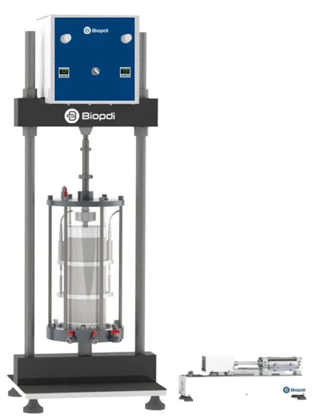
- Pneumatic actuator applies the deviator stress pulses, from 1 to 5 Hz
- Dynamic triaxial cell acrylic and aluminum, air confinement up to 200 kPa
- Pressurization pneumatic, keeps the confining stress constant
- Submersible load cell 20 kN, inside the chamber
- Two displacement sensors submersible, measure the resilient displacement
- Software DNIT 134, 135 and 179 routines, with the MR for each stress pair
Accessories for resilient modulus testing
The accessories below are mounted on the same press, depending on the material and the standard:
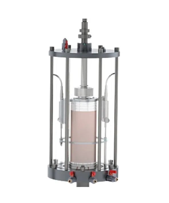 Dynamic triaxial cellsoils and crushed stone, DNIT 134 and 179
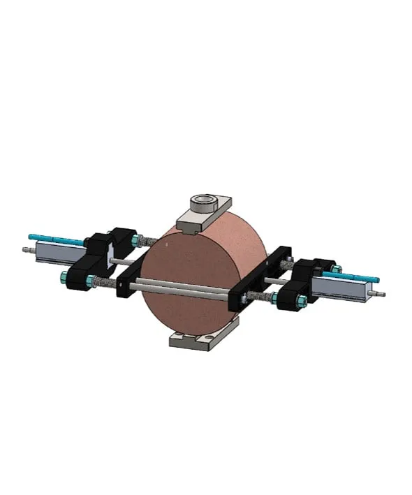 Diametral compressionasphalt mixtures, DNIT 135
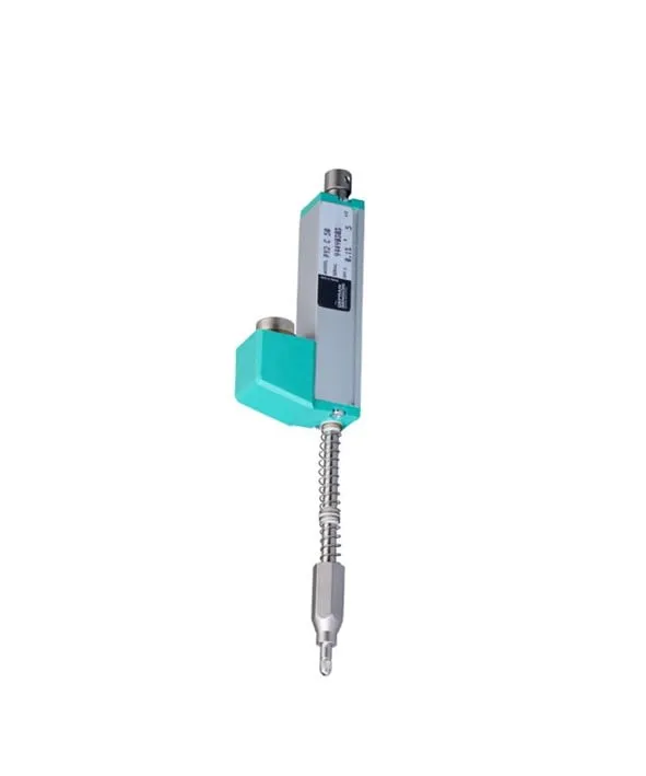 LVDTsubmersible and non-submersible
The press comes in two versions. The basic dynamic triaxial press has the confining pressure set manually on the pneumatic pressurizer regulator and read on the pressure gauge in kPa. The automatic dynamic triaxial press controls the confining pressure automatically. For chemically stabilized materials, the MR DNIT 181 fixture, for 100 mm and 150 mm specimens, holds the pair of 10 mm LVDTs on the middle third of the test specimen (DNIT 181/2018-ME). There is also a model that combines static and dynamic testing, presented on the triaxial testing system page. In the software, the resilient modulus tab shows the resilient displacement and the MR (in kPa) for each stress pair. The permanent deformation tab plots deformation against time and number of cycles. Asphalt mixture specimens are molded separately, as in the Marshall test, for which Biopdi offers the CBR/Marshall test press.
Exercise 5: is the piston capacity enough?
What is the highest load the soil tests demand from the piston, for both specimen sizes?
- The most severe stress pair in DNIT 134 has σd = 0.420 MPa. For the 100 mm cylinder, P = 0.420 × 7,854 = 3,299 N. For the 150 mm cylinder, A = π × 75² = 17,671 mm² and P = 0.420 × 17,671 = 7,422 N.
- The most severe stress pair in DNIT 179 has σd = 360 kPa. For the 150 mm cylinder, P = 0.360 × 17,671 = 6,362 N.
- The highest confining stress in the two tests is 0.140 MPa (1.4 bar). That is below the 200 kPa limit of the dynamic triaxial cell and well below the 10 bar pneumatic supply.
With a 20 kN capacity, the highest load in the soil tests uses just over one third of it (37%), even with the 150 × 300 mm test specimen. To configure the equipment for your materials, request a quote.
Standards cited
The DNIT standards below are listed as current in the DNIT standards collection. The collection was checked on October 1, 2026, and again on October 5, 2026, against the IPR (DNIT's Road Research Institute) standards list dated September 9, 2026. The full texts of the standards that govern MR, tensile strength (RT), fatigue and permanent deformation were also checked. The foreign references are the ones cited in the bibliographies of the Brazilian standards:
| Standard | Subject | Edition |
|---|---|---|
| DNIT 134-ME | resilient modulus of soils and crushed stone, repeated-load triaxial test | 2018, Erratum 1 of 2023 |
| DNIT 135-ME | resilient modulus of asphalt mixtures, diametral compression | 2018 |
| DNIT 179-IE | permanent deformation of soils and crushed stone | 2018, Erratum 1 of 2023 |
| DNIT 136-ME | indirect tensile strength of asphalt mixtures by diametral compression | 2018 |
| DNIT 181-ME | resilient modulus of chemically stabilized materials | 2018, Erratum 1 of 2023 |
| DNIT 183-ME | fatigue of asphalt mixtures by diametral compression | 2018 |
| DNIT 184-ME | permanent deformation resistance of asphalt mixtures, uniaxial repeated-load test (flow number) | 2018 |
| DNIT 143-ES | soil-cement base, construction specification | 2025 |
| IS-247 (DNIT/IPR) | design studies for new highways using MeDiNa | current, supplements IPR Publication 726 |
| DNIT 416-ME | dynamic modulus of asphalt mixtures | 2019 |
| DNIT 443-ME | soil compaction in split (three-part) molds | 2023 |
| AASHTO T 307 | resilient modulus of soils and aggregates (US reference) | cited in DNIT 134 |
| ASTM D7369 | resilient modulus of asphalt mixtures by indirect tension | D7369-20 |
| ABNT NBR 16018 | stiffness of asphalt mixtures by diametral compression under repeated loading | cited in DNIT 135 |
Other tests and technical references
Marshall test: stability, flow, Vv, VMA (VAM) and VFA (RBV) per DNIT 447/2024-ME
The Marshall test measures the stability and flow of asphalt mixtures at 60 °C per DNIT 447/2024-ME. Procedure, Vv, VMA, VFA and a worked example.
CBR test and the California Bearing Ratio
CBR test (California Bearing Ratio): NBR 9895:2025 and DNIT 172 standards, procedure, formula with 6.9 and 10.35 MPa, worked example and CBR by layer.
Triaxial test: what it is, UU, CU and CD types, calculations and standards
What the triaxial test is, what the name means, the UU, CU and CD types with their standards, the B parameter, the formulas and worked CU, UU and CD examples.
Consolidation test (oedometer test): procedure, Cc, σ'vm, cv and settlement per NBR 16853
Consolidation (oedometer) test per Brazilian NBR 16853:2020: measure Cc, σ'vm and cv in load-doubling stages, predict how much and how fast clay settles.
Frequently asked questions
What is resilient modulus?
Resilient modulus is the ratio between the deviator stress applied repeatedly to a soil, crushed stone or asphalt mixture and the strain the material recovers after each pulse: MR = σd/εr, in MPa. It represents the elastic stiffness of the material under traffic and is the stiffness input for mechanistic pavement design.
How do you calculate resilient modulus?
Divide the deviator stress (σd = P/A) by the resilient strain (εr = δr/H0, with the accumulated permanent displacement subtracted from H0). Example: σd = 0.105 MPa and εr = 7.21 × 10⁻⁴ give MR ≈ 146 MPa. For asphalt mixtures, MR = P·(0.2692 + 0.9976·ν)/(ΔH·t), according to DNIT 135/2018-ME.
What is the difference between resilient modulus in pavements and in metals?
They are different quantities with the same name. In metals, the modulus of resilience is the elastic energy per unit volume up to yielding, Ur = σe²/(2E), in J/m³. In pavement engineering, MR = σd/εr is a stiffness under repeated loading, in MPa.
Which standard governs the resilient modulus test?
Soils, crushed stone and materials that are not chemically stabilized follow DNIT 134/2018-ME (repeated-load triaxial test). Asphalt mixtures follow DNIT 135/2018-ME (diametral compression). Chemically stabilized materials follow DNIT 181/2018-ME.
What is the frequency of the resilient modulus test?
1 Hz: a 0.1 s load pulse followed by 0.9 s of rest, in DNIT 134 and 135. The permanent deformation test (DNIT 179/2018-IE) recommends 2 Hz, with 0.1 s of loading and 0.4 s of rest, and allows 1 to 5 Hz.
How many stress pairs does the soil test have?
Three conditioning pairs, with 500 cycles each, followed by 18 pairs for the calculation: six confining stresses from 0.020 to 0.140 MPa, each with σ1/σ3 ratios of 2, 3 and 4. For subgrade, the designer may adopt 12 pairs.
What is the difference between resilient modulus and modulus of elasticity?
The modulus of elasticity is obtained in a static tensile or compression test, as the slope of the linear portion of the stress-strain curve. MR uses repeated loading and only the recoverable part of the strain, and in soils it varies with stress. For a linear elastic material, the two are the same.
What are typical resilient modulus values?
According to the MeDiNa testing guide (DNIT, 2026): asphalt concrete from 2,000 to 12,000 MPa, cement-treated graded crushed stone from 5,000 to 15,000 MPa, granular materials from 100 to 500 MPa and fine-grained subgrade soils from 25 to 200 MPa.
What is the test temperature for asphalt mixtures?
Usually 25 ± 0.5 °C, with the test specimen conditioned for at least 4 h in the temperature chamber before testing, according to DNIT 135/2018-ME. The chamber must hold 10 to 50 °C with 0.5 °C accuracy.
Can I use CBR to estimate resilient modulus?
Only for screening. Correlations such as MR ≈ 10·CBR were derived for other soils, and the MeDiNa guide does not recommend them because the two parameters correlate poorly. For mechanistic design, MR must be tested.
What is the purpose of the CBR test and how does it differ from resilient modulus?
The CBR test (California Bearing Ratio, ISC in Brazil) measures how well a compacted soil resists penetration by a piston at constant speed, compared with a standard crushed stone, and is used in empirical design. MR measures stiffness under repeated loading, with small, recoverable strains, and is used in mechanistic-empirical design (MeDiNa).
Which resilient modulus standard applies to soil-cement?
DNIT 181/2018-ME, which covers the resilient modulus of chemically stabilized materials such as soil-cement and cement-treated graded crushed stone. DNIT 134/2018-ME excludes these materials. Construction of soil-cement bases has its own specification, DNIT 143/2025-ES.
How is resilient modulus used in MeDiNa?
Each layer is assigned either a constant MR or a k1·σ3^k2·σd^k3·θ^k4 model, plus a Poisson's ratio. The program calculates stresses and strains by multilayer elastic analysis and iterates the MR until it converges at the center of the layer.
What is DNIT IS-247?
IS-247 is DNIT's service instruction for design studies of new highways using MeDiNa. It makes MR testing mandatory for the subgrade, borrow sources, graded crushed stone and asphalt mixtures, sets how many samples must be tested and prohibits replacing tests with data from the MeDiNa database.
How many resilient modulus samples does IS-247 require?
For the subgrade, every sample from the boreholes. For borrow sources for base and subbase, 9 samples from different boreholes. For graded crushed stone for base, 3. For chemically stabilized materials, 3, per DNIT 181. For asphalt mixtures, 1 test with 3 samples, per DNIT 135.
What is the modulus of elasticity of soil?
In pavement engineering, soil stiffness is expressed as the resilient modulus, measured under repeated loading per DNIT 134/2018-ME, not as a static modulus of elasticity. There is no single value. The MR of a soil depends on stress, moisture content and density, so it is reported together with a model fitted to the 18 stress pairs.
Do DNIT 145 and 425 cover resilient modulus?
No. DNIT 145/2012-ES specifies tack coats with asphalt binder, and DNIT 425/2020-ME determines the shape index of aggregates using a caliper. The MR standards are DNIT 134, 135 and 181, all from 2018.
How long does the permanent deformation test take?
At least 150,000 cycles per test specimen, which takes 20.8 h each at 2 Hz. With the 9 specimens recommended by DNIT 179/2018-IE, that comes to about 187.5 h, or almost 8 days of machine time.